Bayesian Statistics
7.3 Hypothesis testing, odds ratios and Bayes factors
Hypothesis testing is surprisingly simple within the Bayesian framework. We first need to introduce the way to present the results.
-
Definition 7.3.1 Let \(A\) and \(B\) be events such that \(\P [A\cup B]=1\) and \(A\cap B=\emptyset \). The odds ratio of \(A\) against \(B\) is
\[O_{A,B}=\frac {\P [A]}{\P [B]}.\]
It expresses how much more likely \(A\) is than \(B\). For example, \(O_{A,B}=2\) means that \(A\) is twice as likely to occur than \(B\); if \(O_{A,B}=1\) then \(A\) and \(B\) are equally likely.
Take a Bayesian model \((X,\Theta )\) with parameter space \(\Pi \). We split the parameter space into two pieces: \(\Pi =\Pi _0\cup \Pi _1\) where \(\Pi _0\cap \Pi _1=\emptyset \). We think of two competing hypothesis:
\(\seteqnumber{0}{7.}{4}\)\begin{align*} H_0&:\text { that }\theta \in \Pi _0, \\ H_1&:\text { that }\theta \in \Pi _1, \end{align*} where \(\theta \) represents the true value of the parameter i.e. the value for which our model should (at least, as a good approximation) match up with reality.
-
Definition 7.3.2 The prior odds of \(H_0\) against \(H_1\) is defined to be
\(\seteqnumber{0}{7.}{4}\)\begin{equation} \label {eq:prior_odds} \frac {\P [\Theta \in \Pi _0]}{\P [\Theta \in \Pi _1]}. \end{equation}
Given the data \(x\), the posterior odds of \(H_0\) against \(H_1\) is defined to be
\(\seteqnumber{0}{7.}{5}\)\begin{equation} \label {eq:posterior_odds} \frac {\P [\Theta |_{\{X=x\}}\in \Pi _0]}{\P [\Theta |_{\{X=x\}}\in \Pi _1]}. \end{equation}
Note that the prior odds involve the prior \(\Theta \), and the posterior odds involve the posterior \(\Theta |_{\{X=x\}}\), but otherwise the formulae are identical. We assume implicitly that \(\P [\Theta \in \Pi _0]\) and \(\P [\Theta \in \Pi _1]\) are both non-zero, which by Theorems 2.4.1 and 3.1.2 implies that the same is true for \(\Theta |_{\{X=x\}}\). Note also that the prior and posterior odds are only well defined for proper prior and posterior distributions, or else we cannot make sense of the probabilities above.
It is often helpful to get a feel for how much the data has influenced the result of the test. For these purposes we also define the Bayes factor
\(\seteqnumber{0}{7.}{6}\)\begin{equation} \label {eq:bayes_factor} B=\frac {\text {posterior odds}}{\text {prior odds}}. \end{equation}
Our next lemma shows why \(B\) is important. It is equal to the ratio of the likelihoods of the event \(\{X=x\}\), i.e. of the data that we have, conditional on \(\Theta \in \Pi _0\) and \(\Theta \in \Pi _1\). In other words, \(B\) is the ratio of the likelihood of \(H_0\) compared to \(H_1\).
Proof: We split the proof into two cases, depending on whether the Bayesian model is discrete or absolutely continuous. In the discrete case we have
\[B =\frac {\P [\Theta |_{\{X=x\}}\in \Pi _0]\P [\Theta \in H_1]}{\P [\Theta |_{\{X=x\}}\in \Pi _1]\P [\Theta \in H_0]} =\frac {\frac {\P [\Theta \in \Pi _0, X=x]}{\P [X=x]}\P [\Theta \in H_1]}{\frac {\P [\Theta \in \Pi _1, X=x]}{\P [X=x]}\P [\Theta \in H_0]} =\frac {\frac {\P [\Theta \in \Pi _0,X=x]}{\P [\theta \in \Pi _0]}}{\frac {\P [\Theta \in \Pi _1,X=x]}{\P [\theta \in \Pi _1]}} =\frac {\P [X|_{\{\Theta \in \Pi _0\}}=x]}{\P [X|_{\{\Theta \in \Pi _1\}}=x]}. \]
We have used equation (1.4) from Lemma 1.4.1 several times here. The continuous case is left for you, in Exercise 7.8 ∎
As a rough guide to translating the Bayes factor into common language, the following table1 is sometimes used: \(\seteqnumber{0}{7.}{7}\)
\begin{equation} \label {eq:bayes_factor_table} \begin{tabular}{c|l} Bayes factor & Interpretation: evidence in favour of $H_0$ over $H_1$ \\ \hline 1 to 3.2 & Indecisive / not worth more than a bare mention \\ 3.2 to 10 & Substantial \\ 10 to 100 & Strong \\ above 100 & Decisive \\ \end {tabular} \end{equation}
Note that a high value of \(B\) only says that \(H_0\) should be preferred over \(H_1\). It does not tell us anything objective about how good our model \((M_\theta )\) is; it only tells us that \(X|_{\{\Theta \in \Pi _0\}}\) is a better fit for \(x\) than \(X|_{\{\Theta \in \Pi _1\}}\) is.
Values of the Bayes factor below \(1\) suggest evidence in favour of \(H_1\) over \(H_0\). In such a case we can swap the roles of \(H_0\) and \(H_1\), which corresponds to the Bayes factor changing from \(B\) to \(1/B\), and we can then use the same table to discuss the weight of evidence in favour of \(H_1\) over \(H_0\).
-
Example 7.3.4 Returning to Example 4.5.3, suppose that we wished to test the hypothesis that the speed camera is, on average, overestimating the speed to cars. Recall that in this example:
-
• Our model was the \(N(\mu ,\frac {1}{\tau })\), for the speed recorded by the camera when a car travels at exactly 30mph.
-
• We used a weak prior \((\mu ,\tau )\sim \NGam (30,\frac {1}{10^2},1,\frac 15)\).
-
• We found the posterior \((\mu ,\tau )\sim \NGam (30.14, 10.01, 6.00, 1.24)\).
Both the posterior and prior density functions are plotted in Example 4.5.3.
Recall that if \((\mu ,\tau )\sim \NGam (m,p,a,b)\) then \(\mu |\tau \sim \Normal (m,\frac {1}{p\tau })\), so the marginal mean of \(\mu \) is \(m\). Hence, the speed camera on average overestimates the speed when \(\mu >30\), and underestimates on average when \(\mu <30\). The probability that \(\mu \) is exactly \(30\) is zero, because our posterior \(\NGam \) is a continuous distribution, so we will simply ignore that possibility. We don’t care about the location of \(\tau \) here so we simply allow it to take any value \(\tau \in (0,\infty )\). This gives us hypothesis
\(\seteqnumber{0}{7.}{8}\)\begin{align*} H_0&:\text { that }(\mu ,\tau )\in \Pi _0=(30,\infty )\times (0,\infty ), \\ H_1&:\text { that }(\mu ,\tau )\in \Pi _1=(-\infty ,30)\times (0,\infty ). \end{align*} We want to compute the Bayes factor \(B\). We’ll start with the posterior odds ratio. We have
\(\seteqnumber{0}{7.}{8}\)\begin{equation*} \P [(\mu ,\tau )\in \Pi _0]=\int _{30}^\infty \int _0^\infty f_{\NGam (30.14, 10.01, 6.00, 1.24)}(\mu ,\tau )\,d\tau \,d\mu \approx 0.82, \end{equation*}
computed numerically and rounded to two decimal places. Note that \(\P [(\mu ,\tau )\in \Pi _1]=1-\P [(\mu ,\tau )\in \Pi _0]\), which gives a posterior odds ratio of
\[\frac {\P [\Theta |_{\{X=x\}}\in H_0]}{\P [\Theta |_{\{X=x\}}\in H_1]}=\frac {0.82}{1-0.82}=4.56\]
again rounded to two decimal places. The prior odds ratio, calculated via the same procedure, is exactly \(1\). This occurs because of the symmetry of the prior \(\NGam (30,\frac {1}{10^2},1,\frac 15)\) distribution (this symmetry is visible in the sketch in Example 4.5.3) gives that \(\P [\NGam (30,\frac {1}{10^2},1,\frac 15)\in \Pi _1]=\P [\NGam (30,\frac {1}{10^2},1,\frac 15)\in \Pi _0]=\frac 12\). Hence the Bayes factor for this hypothesis test is
\(\seteqnumber{0}{7.}{8}\)\begin{equation} B=\frac {4.56}{1.00}=4.56. \end{equation}
Based on table (7.8), we have substantial evidence that the speed camera is overestimating speeds.
A potential problem with our test is that we have not cared about how much the camera is overestimating speeds. The (marginal) mean of \(\mu \) in our posterior distribution is \(30.14\), which is only slightly larger than the true speed \(30\), and this suggests that the error is fairly small. We would need to be careful about communicating the result of our test, to avoid giving the wrong impression.
Note that we have used a small amount of Bayesian shorthand in this example, by writing \(\mu \) and \(\tau \) for both random variables and samples of these random variables.
-
7.3.1 Comparison to classical hypothesis testing
The endpoint of a Bayesian hypothesis test is usually a Bayes factor \(B\) which can then be interpreted, using table (7.8) or similar, into common language that describes the strength of evidence in favour of \(H_0\) over \(H_1\). There is no ‘pass’ or ‘fail’ outcome, just a comparison between two situations.
You will have seen a different method of carrying out a hypothesis test before, looking something like this.
-
Definition 7.3.5 \(\offsyl \) The classical hypothesis test is the following procedure:
-
1. Choose a model family \((M_\theta )_{\theta \in \Pi }\), choose a value \(\theta _0\in \Pi \) and define \(H_0\) to be the model \(M_{\theta _0}\). This is often written in shorthand as \(H_0:\theta =\theta _0\).
-
2. Calculate a value \(p\) as follows. Assume that \(H_0\) is true i.e. use the model \(M_{\theta _0}\) and using this model, calculate \(p\) to be the probability of observing data that is (in some chosen sense) ‘at least as extreme’ as the data \(x\) that we actually observed.
If \(p\) is sufficiently small (in some chosen sense) then reject \(H_0\).
-
Let us think about this process carefully. Firstly, there is no need for an ‘alternative hypothesis’ in Definition 7.3.5. More specifically, rejecting \(H_0\) means that we think it is unlikely that our chosen model \(M_{\theta _0}\) would generate the data \(x\), so consequently we think it is unlikely that \(M_{\theta _0}\) is a good model.
There is nothing else to say here! Rejecting \(H_0\) does not mean that the ‘alternative hypothesis’ \(H_1\) that \(\theta \neq \theta _0\) is accepted (or true). If \(p\) turns out to be small it means that either (i) \(M_{\theta _0}\) is a good model and our data \(x\) was unlikely to have occurred or, (ii) \(M_{\theta _0}\) is a bad model for our data. Neither statement tells us what a good model might look like. Unfortunately classical hypothesis testing is very often misunderstood, and rejection of \(H_0\) is incorrectly treated as though it implies that \(H_1\) is true.
If we do not reject \(H_0\), then it means that the model \(M_{\theta _0}\) is reasonably likely to generate the data we have. This leaves open the possibility that there may be lots of other models, not necessarily within our chosen model family, that are also reasonably likely to generate the data we have. This point is sometimes misunderstood too.
There are several other common mistakes that are based on misunderstanding the role of a \(p\)-values. For example, you may come across claims that the \(p\)-value is the probability that \(H_0\) is true, or that \(H_1\) is false, or that it is the probability that the data occurred via ‘random chance’. None of these things match step 2 of Definition 7.3.5. A further issue is \(p\)-hacking, which refers to carrying out repeated tests (with new data each time) and then only reporting the experiments that rejected \(H_0\). This amounts to rejection sampling, conditioning the model on the event that it generates unusual data, which changes the model and invalidates the test.
In summary, the main problem with Definition 7.3.5 is that understanding the outcome of a classical hypothesis test requires careful logic, which opens a door both to human error and to misuse. The Bayesian hypothesis test is comparatively easy to interpret.
-
Example 7.3.6 \(\offsyl \) A famous example of one of these mistakes comes from the ‘clever Hans’ effect. Hans was a horse who appeared to be able to do arithmetic, owned by a mathematics teacher Wilhelm von Osten. Von Osten would ask Hans (by speaking out loud) to answer to various questions and Hans would reply by tapping his hoof. The number of taps was interpreted as a numerical answer. Hans answered the vast majority of questions correctly.
To construct a hypothesis test using Definition 7.3.5, take a model family \(M_{\theta }\sim \Bern (\theta )^{\otimes n}\), where the data \(x=(x_1,\ldots ,x_n)\) corresponds to \(x_i=1\) for solving the \(n^{\text {th}}\) question correctly, and \(x_i=0\) for incorrectly. We don’t know exactly how hard the arithmetic questions were, so let us suppose that the probability of Hans solving a question correctly by guessing at random is \(\theta =\frac 12\) (this is clearly a very generous assumption for arithmetic). So, take
\[H_0:\text { that }\theta =1/2\;\text { i.e.~the horse solves the questions at random}\]
and then the model we wish to test is \(M_{\frac 12}\). The horse is asked \(n=10\) questions, and it answers them all correctly. Our model \(M_{\frac 12}\) says the probability of this is \((\frac 12)^{10}\approx 0.001=p\). We reject \(H_0\). Taking any value \(\theta \leq \frac 12\) will lead to the same conclusion.
So, we expect that our model \(M_{\theta }\) is a bad description of reality, for each \(\theta \leq \frac 12\). This does not mean that we must accept \(H_1\) and believe the horse is doing arithmetic i.e. that some alternative model \(M_\theta \) is correct for some larger value of \(\theta \). In fact, what is going on here is that Hans has learnt to read the body language of Wilhelm von Osten, who leans in forwards whilst Hans is tapping his hoof and leans back upright as soon as the correct number of taps has been reached. This was established by the psychologist Oskar Pfungst, who tested Hans and von Osten under several different conditions in a laboratory.
In short, our model that the horse ‘solves’ questions is a bad choice. The horse answers questions correctly but it does not solve questions. To distinguish between these two situations we need a better model than \((M_\theta )\), as Pfungst did in his laboratory. His model included (amongst other things) an extra variable for whether Hans could see von Osten.
After the investigations by Pfungst were done, von Osten refused to believe what Pfungst had discovered, and continued to show Hans around Germany. They attracted large and enthusiastic crowds, and made a substantial amount of money from doing so – many in his audience wondered if they should accept \(H_1\).
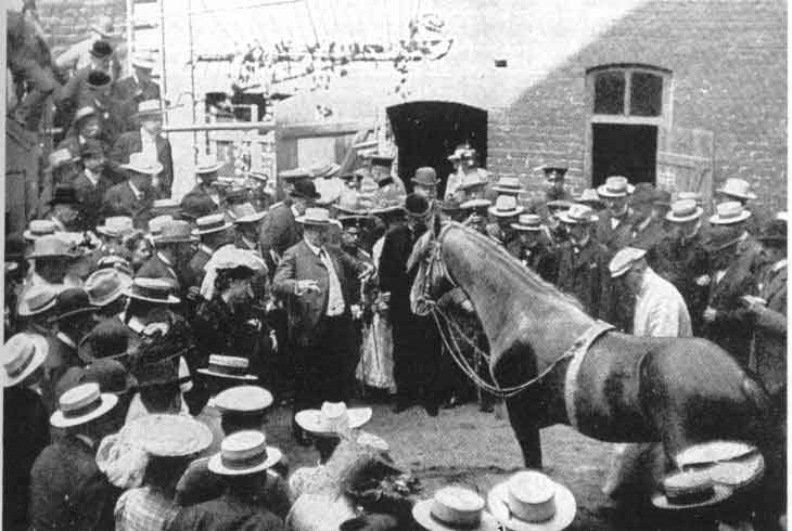
Figure 7.1: Hans the horse in 1904, correctly answering arithmetic questions set by his owner Wilhem von Osten.