Bayesian Statistics
Chapter 7 The posterior
After carrying out one or more Bayesian updates, the key piece of information that we obtain is the posterior distribution \(\Theta |_{\{X=x\}}\). In this chapter we analyse the posterior and discuss standard methods of presenting Bayesian analysis. Throughout this chapter we work in the situation of a discrete or continuous Bayesian model \((X,\Theta )\), where we have data \(x\) and posterior \(\Theta |_{\{X=x\}}\). We keep all of our usual notation: the parameter space is \(\Pi \), the model family is \((M_\theta )_{\theta \in \Pi }\), and the range of the model is \(R\). Note that \(M_\theta \) could have the form \(M_\theta \sim (Y_\theta )^{\otimes n}\) for some random variable \(Y_\theta \) with parameter \(\theta \), corresponding to \(n\) i.i.d. data points.
We have noted in Chapter 5 that a well chosen prior distribution can lead to a more accurate posterior distribution, but a poorly chosen posterior can also harm the analysis. If different perspectives are involved then the specification of prior beliefs can become complicated. For example, trials of medical treatments involve patients, pharmaceutical companies and regulators, all of whom have different levels of trust in each other as well as potentially different prior beliefs. It is common practice to check how much the posterior distribution depends upon the choice of prior, often by varying the prior or comparing to a weakly informative prior.
7.1 Credible intervals
In this section we look at interval estimates for the unknown parameter \(\theta \). The key term used in the Bayesian framework is the following definition.
-
Definition 7.1.1 A credible interval is a subset \(\Pi _0\sw \Pi \) that is chosen to minimize the size of \(\Pi _0\) and maximize \(\P [\Theta |_{\{X=x\}}\in \Pi _0]\).
This is a practical definition rather than a mathematical one: we must choose how to balance the minimization of \(\Pi _0\) against maximization of \(\P [\Theta |_{\{X=x\}}\in \Pi _0]\) as best we can, and in some situations there is no single right answer. They are also sometimes known as high posterior density regions, usually shortened to HPDs or HDRs.
-
Example 7.1.2 Suppose that our posterior has come out as \(\Theta |_{\{X=x\}}\sim \Normal (0,1.5^2)\).
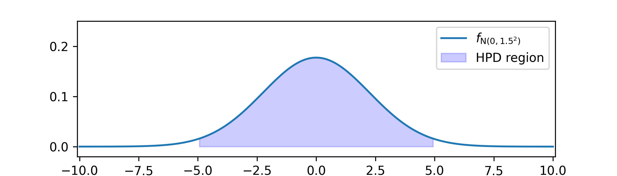
We choose our credible interval to be \([-5,5]\). This region is much smaller than the range of \(\Theta \), which is the whole of \(\R \). The probability that it contains \(\Theta |_{\{X=x\}}\) is given by \(\P [-5\leq N(0,1.5^2)\leq 5]\approx 0.97\).
More generally, if we are dealing with a continuous distribution with a single peak then it is common to choose a credible interval of the form \(\Pi _0=[a,b]\) where
\(\seteqnumber{0}{7.}{0}\)\begin{equation} \label {eq:hpd_eq_tails_prob} \P \l [\Theta |_{\{X=x\}}<a\r ]=\P \l [\Theta |_{\{X=x\}}>b\r ]=\frac {1-p}{2} \end{equation}
and some value is picked for \(p\in (0,1)\). Credible intervals of this type are said to be equally tailed. They always contain the mode of \(\Theta |_{\{X=x\}}\), and from (7.1) we have \(\P [\Theta |_{\{X=x\}}\in [a,b]]=p\). By symmetry the credible interval in Example 7.1.2 is equally tailed, and we will give an asymmetric case in Example 7.1.3.
A value of \(p\) close to \(1\) gives a wide interval and a high value for \(\P [\Theta |_{\{X=x\}}\in [a,b]]\), whilst a value of \(p\) close to \(0\) gives a thinner interval but a lower value for \(\P [\Theta |_{\{X=x\}}\in [a,b]]\). As in Example 7.1.2, we want to choose \(p\in (0,1)\) to make \([a,b]\) thin and make \(\P [\Theta |_{\{X=x\}}\in [a,b]]\) large, if possible.
-
Example 7.1.3 Suppose that our posterior has come out as \(\Theta |_{\{X=x\}}\sim \Gam (4,3)\). We want an equally tailed credible interval region \([a,b]\) such that \(\P [\Theta |_{\{X=x\}}\in [a,b]]=0.8\).
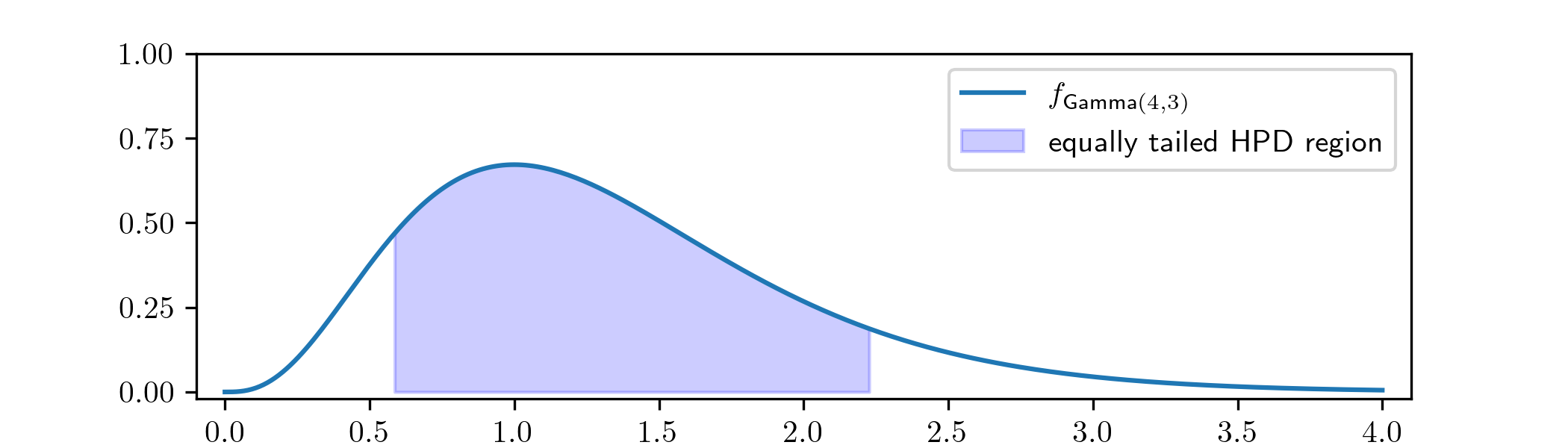
The region is chosen by finding \(a\) such that \(\P [\Theta |_{\{X=x\}}<a]=\frac {1-0.8}{2}=0.1\) and \(b\) such that \(\P [\Theta |_{\{X=x\}}>b]=\frac {1-0.8}{2}=0.1\). These values were found numerically to be \(a=0.58\) and \(b=2.23\), to two decimal places. You can find the code that generated this example as part of Exercise 7.5.
-
Remark 7.1.4 \(\offsyl \) It is possible to construct a form of hypothesis testing based on credible intervals. For example, we might by choose an equally tailed credible interval \(\Pi _0\) with a \(95\%\) probability of containing \(\Theta |_{\{X=x\}}\), and then we then reject the hypothesis \(\theta =\theta _0\) if and only if \(\theta _0\notin \Pi _0\). This approach is known as Lindley’s method.
We can define credible intervals for the prior in the same ways as detailed above, with \(\Theta \) in place of \(\Theta |_{\{X=x\}}\). These are less useful for parameter estimation although they can be useful for prior elicitation. They are sometimes known as high prior density regions. We implicitly used equally tailed regions of this type in Example 5.1.1, when we asked an elicitee to estimate their 25th and 75th percentiles.
7.1.1 Credible intervals vs confidence intervals
I think it is fair to say that many - perhaps even, most - users of confidence intervals could not tell you from memory what a confidence interval is. The formal definition of a confidence interval is the following.
-
Definition 7.1.5 \(\offsyl \) Given a model family \((M_\theta )_{\theta \in \Pi }\) with range \(R\), a confidence interval with confidence level \(\alpha \) is a pair of deterministic functions \(u(\cdot )\) and \(v(\cdot )\) defined from \(R\) to \(\R \) such that \(\P [u(M_\theta )<\theta <v(M_\theta )]=\alpha \) for all \(\theta \in \Pi .\)
The point of this definition is that, for the true parameter value \(\theta ^*\) and some observed data \(Y\) that (if our model is good) satisfies \(y\sim M_{\theta ^*}\), then without knowing \(\theta ^*\) we can write down an interval \([u(Y),v(Y)]\) for which \(\P [u(Y)<\theta ^*<v(Y)]=\alpha \).
For example, if \(Y\sim M_\theta \sim \Normal (\theta ,\sigma ^2)\), where \(\sigma \) is known, then \(\P [Y-2\sigma <\theta <Y+2\sigma ]=\P [\theta -2\sigma <Y<\theta +2\sigma ]\approx 0.95\) so \([Y-2\sigma ,Y+2\sigma ]\) is a 95% confidence interval. If we have data \(y\sim M_{\theta ^*}\) that we believe was sampled from the model (with its true parameter value) then we might say that \([y-2\sigma ,y+2\sigma ]\) is a 95% confidence interval.
We now have enough background to discuss how confidence intervals compare to credible intervals:
-
• Confidence intervals and credible intervals are different objects: the easiest way to see this is by noting that in Definition 7.1.5 the parameter \(\theta \) is deterministic and the data is random, whereas in a Bayesian model the parameter and the data are both random variables.
This is a subtle point that is easily misunderstood. Many people find the idea of a credible interval more natural, so amongst non-experts you will often see a confidence interval misinterpreted as though it is a credible interval.
-
• Both confidence intervals and credible intervals are based on the assumption that, for some true parameter value \(\theta ^*\), the model \((M_\theta )\) accurately represents the real-world situation that generates the data. Confidence intervals are entirely reliant on this assumption, whereas for credible intervals the prior (of the underlying Bayesian model) also has an influence. The key advantage of credible intervals is that, with an informative prior \(\Theta \), we could obtain an credible interval that is significantly smaller than the confidence interval generated by the same model family.
For example, in early stages of clinical trails of drugs that treat rare conditions (making it difficult to find participants), expert opinion concerning side effects has been used as a prior alongside the experimental data, leading to approval of drugs that would not otherwise have demonstrated enough evidence of safety.
-
• In many situations, particularly when there is plenty of data available (in which case the influence of the prior is diminished), it is possible to prove that confidence intervals and credible intervals are approximately equal.
7.1.2 A little history \(\offsyl \)
You will sometimes find that statisticians describe themselves as ‘Bayesian’ or ‘frequentist’, carrying the implication that they prefer to use one family of methods over the other. This may come from greater experience with one set of methods or from a preference due to the specifics of a particular model. A technique is said to be ‘frequentist’ if it relies only on repeated sampling of data, rather than e.g. eliciting a prior. A confidence interval is an example of a frequentist technique.
To a great extent this distinction is historical. During the middle of the 20th century statistics was dominated by frequentist methods, because they could be implemented for complex models without the need for modern computers. Once it was realized that modern computers made Bayesian methods possible, the community that investigated these techniques needed a name and an identity, to distinguish itself as something new. The concept of identifying as ‘Bayesian’ or ‘frequentist’ is essentially a relic of that social process, rather than anything with a clear mathematical foundation.
Modern statistics makes use of both Bayesian and non-Bayesian methods to estimate parameters. Sometimes it mixes the two approaches together or chooses between them for model-specific reasons. We do need to divide things up in order to learn them, so will only study Bayesian models within this course – but in general you should maintain an understanding of other approaches too.