Bayesian Statistics
7.2 The connection to maximum likelihood
You have already seen maximum likelihood based methods for parameter inference in previous courses.
-
Definition 7.2.1 Let \((M_\theta )\) be a model family with range \(R\) and let \(x\in \R \). The maximum likelihood estimator of \(\theta \) given the data \(x\) is
\(\seteqnumber{0}{7.}{1}\)\begin{equation} \label {eq:mle_def} \hat {\theta }=\argmax _{\theta \in \Pi } L_{M_\theta }(x) \end{equation}
The value of \(\hat \theta \) is usually uniquely specified by (7.2). Graphically, it is the value of \(\theta \) corresponding to the highest point on the graph \(\theta \mapsto L_{M_\theta }(x)\). Heuristically, it is the value of \(\theta \) that produces a model \(M_\theta \) that has the highest probability (within our chosen model family) to generate the data that we actually saw.
Definition 7.2.1 might remind you of a simpler concept that applies to a single random variable. Recall that, for a discrete random variable \(Y\), the mode is most likely single value for \(Y\) to take, or \(\argmax _{y\in R_Y} \P [Y=y]\) in symbols. For a continuous random variable \(Y\), with range \(R_Y\), the mode of \(Y\) is the value \(y\in R_Y\) that maximises the p.d.f. \(f_Y(y)\), given by \(\argmax _{y\in R_Y}f_Y(x)\). Putting these two cases together, in general the mode is \(\argmax _{y\in R_Y}L_Y(y)\).
-
Example 7.2.2 For continuous random variables, \(\P [Y=y]=0\) for all \(y\). The idea in this case is that the concept of ‘most likely value’ is best represented by the maximum of the probability density function. Let \(Y\sim \Gam (3,4)\), with p.d.f.
\[f_Y(y)=\begin {cases} 32y^{2}e^{-3y} & \text { for }y>0,\\ 0 & \text { otherwise.} \end {cases} \]
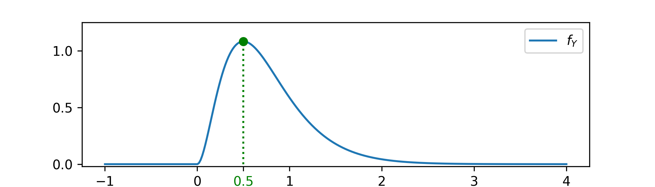
The mode is shown at its value \(y=\frac 12\). This value can be found by solving the equation \(\frac {df_Y(y)}{dy}=32\l (2ye^{-4y}+y^2(-4e^{-4y})\r )=32ye^{-4y}(2-4y)=0\) and checking that the solution \(y=\frac 12\) corresponds to a local maxima.
Bayes’ rule (6.3) says that
\[f_{\Theta |_{\{X=x\}}}(\theta )\propto L_{M_\theta }(x)f_\Theta (\theta ).\]
Comparing this equation to (7.2), we can extract a clear connection between MLEs and Bayesian inference. More precisely, the MLE approach can be viewed as a simplification of the Bayesian approach. There are two steps to this simplification:
-
1. Fix the prior to be a uniform distribution (or an improper flat prior, if necessary).
With this choice, for \(\theta \in \Pi \) we obtain the posterior density
\(\seteqnumber{0}{7.}{2}\)\begin{equation} \label {eq:posterior_from_flat_prior} f_{\Theta |_{\{X=x\}}}(\theta )\propto L_{M_\theta }(x). \end{equation}
-
2. Then, instead of considering the posterior distribution as a random variable, we approximate the posterior distribution with a point estimate: its mode.
Comparing (7.3) to (7.2), this mode is precisely the maximum likelihood estimator \(\hat \theta \).
In principle we might make either one of these simplifications without the other one, but they are commonly made together.
We now have enough background to discuss how MLEs compare to Bayesian inference:
-
• We’ve seen in many examples that, as the amount of data that we have grows, the posterior distribution tends to become more and more concentrated around a single value. In such a case, the MLE becomes a good approximation for the posterior. This situation is common when we have plenty of data – see Section 7.2.1 for a more rigorous (but off-syllabus) discussion.
-
• If we do not have lots of data then the approximation in step 2 will be less precise and the influence of the prior will matter. In this case a well chosen prior can lead to significantly more informative analysis.
In general we should be careful about approximating the posterior distribution with a single number (e.g. the mean, median or mode), especially if the distribution is not concentrated within a small region. We might lose valuable information by doing so.
-
• If our model family \((M_\theta )\) is not a reasonable reflection of reality then both methods become unreliable – no matter how much data we have.
7.2.1 Making the connection precise \(\offsyl \)
Several theorems are known which actually prove, under wide ranging conditions, that when we have plenty of data the MLE and Bayesian approaches become essentially equivalent. These theorems are complicated to state, but let us give a brief explanation of what is known here.
Take a model family \((M_\theta )_{\theta \in \Pi }\) and define a Bayesian model \((X,\Theta )\) with model family \(M_\theta ^{\otimes n}\). This model family represents \(n\) i.i.d. samples from \(M_\theta \). Fix some value \(\theta ^*\in \Pi \), which we think of as the true value of the parameter \(\theta \). Let \(x\) be a sample from \(M_{\theta ^*}^{\otimes n}\). We write the posterior \(\Theta |_{\{X=x\}}\) as usual.
Let \(\hat \theta \) be the MLE associated to the model family \(M_\theta ^{\otimes n}\) given the data \(x\), that is \(\hat \theta =\argmax _{\theta \in \Pi }L_{M_\theta ^{\otimes n}}(x)\). Then as \(n\to \infty \) it holds that
\(\seteqnumber{0}{7.}{3}\)\begin{equation} \label {eq:bvm} \Theta |_{\{X=x\}}\approxd \Normal \l (\theta ^*,\frac {1}{n}I(\theta ^*)^{-1}\r ) \approxd \Normal \l (\hat {\theta },\frac {1}{n}I(\theta ^*)^{-1}\r ) \end{equation}
where \(I(\theta )\) is the Fisher information matrix defined by \(I(\theta )_{ij}=\E [\frac {\p ^2}{\p \theta _i \theta _j}\log f_{M_\theta }(X_1)]\) (where \(X_1\) has the distribution \(M_\theta \)). The key point is that (7.4) says that the posterior \(\Theta |_{\{X=x\}}\), the MLE \(\theta ^*\) and the true parameter value \(\theta ^*\) are in fact very similar, for large \(n\), because of the factor \(\frac 1n\) in the variance.
The left hand equality of (7.4) is known as the Bernstein von-Mises theorem. The first rigorous proof was given by Doob in 1949 for the special case of finite sample spaces. It has since been extended under more general assumptions that we won’t detail here. Examples are also known where it fails to hold for some choices of prior distribution, although this behaviour is rare in practice. Right right hand equality in (7.4) is known as the asymptotic efficiency of MLEs and is another important theorem in advanced statistics.