Stochastic Processes and Financial Mathematics
(part two)

$\newcommand{\footnotename}{footnote}$ $\def \LWRfootnote {1}$ $\newcommand {\footnote }[2][\LWRfootnote ]{{}^{\mathrm {#1}}}$ $\newcommand {\footnotemark }[1][\LWRfootnote ]{{}^{\mathrm {#1}}}$ $\let \LWRorighspace \hspace $ $\renewcommand {\hspace }{\ifstar \LWRorighspace \LWRorighspace }$ $\newcommand {\mathnormal }[1]{{#1}}$ $\newcommand \ensuremath [1]{#1}$ $\newcommand {\LWRframebox }[2][]{\fbox {#2}} \newcommand {\framebox }[1][]{\LWRframebox } $ $\newcommand {\setlength }[2]{}$ $\newcommand {\addtolength }[2]{}$ $\newcommand {\setcounter }[2]{}$ $\newcommand {\addtocounter }[2]{}$ $\newcommand {\arabic }[1]{}$ $\newcommand {\number }[1]{}$ $\newcommand {\noalign }[1]{\text {#1}\notag \\}$ $\newcommand {\cline }[1]{}$ $\newcommand {\directlua }[1]{\text {(directlua)}}$ $\newcommand {\luatexdirectlua }[1]{\text {(directlua)}}$ $\newcommand {\protect }{}$ $\def \LWRabsorbnumber #1 {}$ $\def \LWRabsorbquotenumber "#1 {}$ $\newcommand {\LWRabsorboption }[1][]{}$ $\newcommand {\LWRabsorbtwooptions }[1][]{\LWRabsorboption }$ $\def \mathchar {\ifnextchar "\LWRabsorbquotenumber \LWRabsorbnumber }$ $\def \mathcode #1={\mathchar }$ $\let \delcode \mathcode $ $\let \delimiter \mathchar $ $\def \oe {\unicode {x0153}}$ $\def \OE {\unicode {x0152}}$ $\def \ae {\unicode {x00E6}}$ $\def \AE {\unicode {x00C6}}$ $\def \aa {\unicode {x00E5}}$ $\def \AA {\unicode {x00C5}}$ $\def \o {\unicode {x00F8}}$ $\def \O {\unicode {x00D8}}$ $\def \l {\unicode {x0142}}$ $\def \L {\unicode {x0141}}$ $\def \ss {\unicode {x00DF}}$ $\def \SS {\unicode {x1E9E}}$ $\def \dag {\unicode {x2020}}$ $\def \ddag {\unicode {x2021}}$ $\def \P {\unicode {x00B6}}$ $\def \copyright {\unicode {x00A9}}$ $\def \pounds {\unicode {x00A3}}$ $\let \LWRref \ref $ $\renewcommand {\ref }{\ifstar \LWRref \LWRref }$ $ \newcommand {\multicolumn }[3]{#3}$ $\require {textcomp}$ $\newcommand {\intertext }[1]{\text {#1}\notag \\}$ $\let \Hat \hat $ $\let \Check \check $ $\let \Tilde \tilde $ $\let \Acute \acute $ $\let \Grave \grave $ $\let \Dot \dot $ $\let \Ddot \ddot $ $\let \Breve \breve $ $\let \Bar \bar $ $\let \Vec \vec $ $\DeclareMathOperator {\var }{var}$ $\DeclareMathOperator {\cov }{cov}$ $\DeclareMathOperator {\indeg }{deg_{in}}$ $\DeclareMathOperator {\outdeg }{deg_{out}}$ $\newcommand {\nN }{n \in \mathbb {N}}$ $\newcommand {\Br }{{\cal B}(\R )}$ $\newcommand {\F }{{\cal F}}$ $\newcommand {\ds }{\displaystyle }$ $\newcommand {\st }{\stackrel {d}{=}}$ $\newcommand {\uc }{\stackrel {uc}{\rightarrow }}$ $\newcommand {\la }{\langle }$ $\newcommand {\ra }{\rangle }$ $\newcommand {\li }{\liminf _{n \rightarrow \infty }}$ $\newcommand {\ls }{\limsup _{n \rightarrow \infty }}$ $\newcommand {\limn }{\lim _{n \rightarrow \infty }}$ $\def \ra {\Rightarrow }$ $\def \to {\rightarrow }$ $\def \iff {\Leftrightarrow }$ $\def \sw {\subseteq }$ $\def \wt {\widetilde }$ $\def \mc {\mathcal }$ $\def \mb {\mathbb }$ $\def \sc {\setminus }$ $\def \v {\textbf }$ $\def \p {\partial }$ $\def \E {\mb {E}}$ $\def \P {\mb {P}}$ $\def \R {\mb {R}}$ $\def \C {\mb {C}}$ $\def \N {\mb {N}}$ $\def \Q {\mb {Q}}$ $\def \Z {\mb {Z}}$ $\def \B {\mb {B}}$ $\def \~{\sim }$ $\def \-{\,;\,}$ $\def \|{\,|\,}$ $\def \qed {$\blacksquare $}$ $\def \1{\unicode {x1D7D9}}$ $\def \cadlag {c\`{a}dl\`{a}g}$ $\def \p {\partial }$ $\def \l {\left }$ $\def \r {\right }$ $\def \F {\mc {F}}$ $\def \G {\mc {G}}$ $\def \H {\mc {H}}$ $\def \Om {\Omega }$ $\def \om {\omega }$ $\def \Vega {\mc {V}}$

11.2 Brownian motion

To work with Brownian motion mathematically, we need more than the pictures from the previous section. What we need is a theorem that (1) tells us that Brownian motion exists and (2) gives us some properties to work with. We begin our mathematical treatment of Brownian motion as follows, with a definition that it also an existence theorem:

Theorem 11.2.1 There is a stochastic process $(B_t)$ such that:
- 1. The paths of $(B_t)$ are continuous.
- 2. For any $0\leq u\leq t$, the random variable $B_t-B_u$ is independent of $\sigma (B_v\-v\leq u)$.
- 3. For any $0\leq u \leq t$, the random variable $B_t-B_u$ has distribution $N(0,t-u)$.
Further, any stochastic process which satisfies these three conditions has the same distribution as $(B_t)$.

Definition 11.2.2 If $B_0=0$ we say that $(B_t)$ is a standard Brownian motion.

From now on we fix some notation, which we will use for the remainder of the course:

We write $(B_t)$ for a standard Brownian motion, and $\mc {F}_t=\sigma (B_u\-u\leq t)$ for its generated filtration. We work over the filtered space $(\Omega ,\mc {F},(\mc {F}_t),\P )$.

Let us record a few simple facts about standard Brownian motion that we will use repeatedly in later chapters. Putting $u=0$ into the second property and noting that $B_0=0$, we obtain that the distribution of Brownian motion at time $t$ is $B_t\sim N(0,t)$. Hence, also,

\[\E [B_t]=0\]

for all $t$. In exercise 11.4 you are are asked to show that if $Z\sim N(0,t)$ then $\E [Z^2]=t$. Hence

\begin{equation} \label {eq:bm_E2} \E [B_t^2]=\var (B_t)=t \end{equation}

for all $t$. It is also useful to know that $B_t^n\in L^1$ for all $n\in \N $. See exercise 11.4 for a proof of this fact.

Along the same lines, another formula that we will use repeatedly (and that you should remember) is that if $Z\sim N(\mu ,\sigma ^2)$ then

\begin{equation} \label {eq:lognormal_mean} \E [e^Z]=e^{\mu +\frac 12\sigma ^2}. \end{equation}

This formula turns out to be surprisingly useful in situations involving Brownian motion. It is proved as part of exercise 11.5.

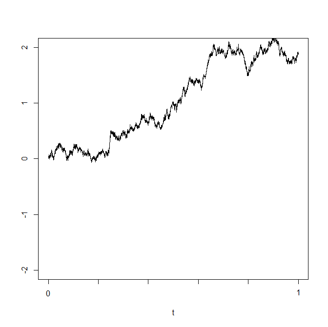
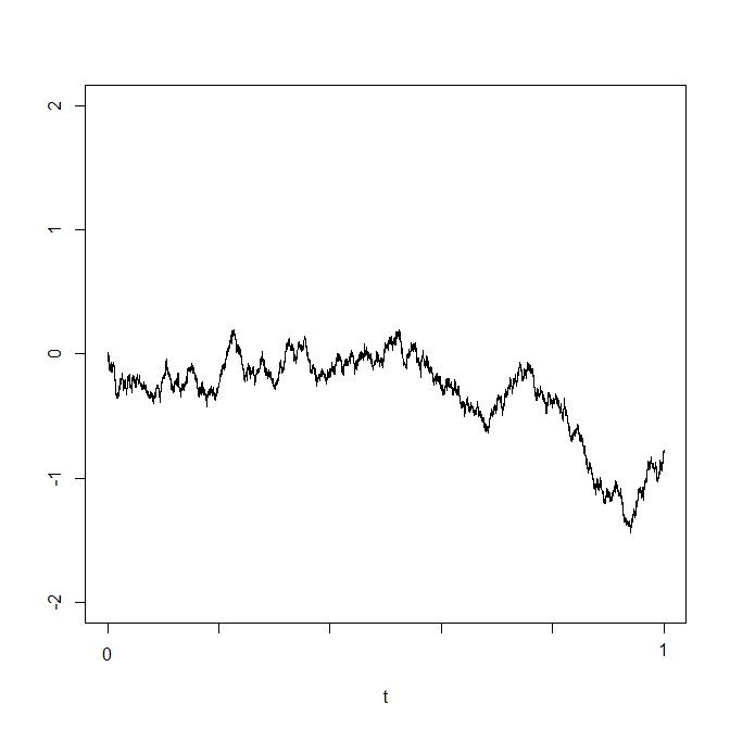
Here are a couple of samples of (standard) Brownian motion. They look very similar in character to the pictures from Section 11.1, when $T$ was large. The key point is that, now, instead of large $T$, time and space have been rescaled so as we only watch $1$ unit of time.

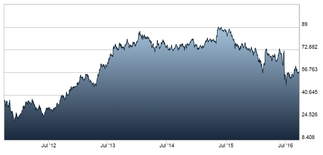
You might like to note the similarity of these pictures to the jagged nature of Figure 1.1 (which was a plot of the stock price of Lloyds Banking Group), which we reproduce here for convenience:

In fact, we won’t use Brownian motion for our stock price model; we’ll use a slight modification known as ‘geometric’ Brownian motion. For now, we need to collect together some more information about Brownian motion, and develop our modelling tools further, but we’ll return to the question of stock price models in Section 13.2 and Chapter 15.

Stochastic Processes and Financial Mathematics (part two)

11.2 Brownian motion

Stochastic Processes and Financial Mathematics
(part two)