Stochastic Processes and Financial Mathematics
(part two)

17.4 Volatility \(\offsyl \)

Let us begin to think a little about what we would need to do to make use of the model, within a real market.

It is clear that we would need estimates of the parameters \(r\) and \(\sigma \) (we don’t need to know \(\mu \), because it has no effect on arbitrage free prices). Estimating the interest rate \(r\) is often rather easy, because interests rates don’t change quickly and they are chosen by banks, who generally also make them public information; so we won’t worry about \(r\).

It is much harder to estimate the volatility \(\sigma \). We focus on this issue for the remainder of this section.

Historical volatility \(\offsyl \)

One obvious idea is to estimate the future volatility based on the stock prices that we have observed in the recent past. Let us discuss one method for doing so.

Recall that our stock price process follows

\[dS_t=\mu S_t\,dt+\sigma S_t\,dB_t\]

which, as we saw in Section 13.2, has solution

\[S_t=S_0\exp \l ((\mu -\tfrac 12\sigma ^2)t+\sigma B_t\r ).\]

We fix \(\epsilon >0\) and set \(t_i=i\epsilon \). We look at our historical data and find the values of \(S_t\) at times \(t=t_i\), which we assume to all be in the past. Fix some \(n\in \N \) and for \(i=1,\ldots ,n\) define

\[\xi _i=\log \l (\frac {S_{t_i}}{S_{t_{i-1}}}\r ).\]

This gives us that

\[\xi _i=\l (\mu -\frac {\sigma ^2}{2}\r )\epsilon + \sigma \l (B_{t_i}-B_{t_{i-1}}\r ).\]

Using the independence properties of Brownian motion, we have that the \((\xi _i)_{i=1}^n\) are i.i.d. random variables with common distribution

\[N\l [(\mu -\tfrac {\sigma ^2}{2})\epsilon ,\;\sigma ^2\epsilon \r ].\]

We can estimate their (common) variance \(\epsilon \sigma ^2\) by the sample variance:

\[\epsilon \sigma ^2 \approx \frac {1}{n-1}\sum \limits _{i=1}^n\l (\xi _i-\bar \xi \r )^2\]

where \(\bar \xi =\frac {1}{n}\sum _{i=1}^n \xi _i\).

We thus obtain the estimator

\[\hat \sigma =\frac {1}{\sqrt {\epsilon }}\l (\frac {1}{n-1}\sum \limits _{i=1}^n (\xi _i-\bar \xi )^2\r )^{1/2}\]

for \(\sigma \). What we have obtained here is a estimate of what the volatility was during the time period containing \(t_1,\ldots ,t_n\), which is in the past. When we are pricing options, what we would like to is an estimator of the volatility for future. We might be prepared to assume that the future will be similar to the past, and if we are then we can use \(\hat \sigma \). Unfortunately, historical volatilities often turn out to be a poor method of predicting future volatilities. With this in mind, we move on and examine an alternative idea.

Implied volatility and the volatility smile \(\offsyl \)

Suppose that we wish to gauge what the (rest of the) market thinks is a reasonable estimate for volatility over the next, say, six months. Here’s one way we could do it.

Take our Black-Scholes model. Find the pricing formula for a European call option that has a date of exercise six months into the future. Let us write this price as \(c(K,t,T,r,\sigma )\). We know the value today of the stock \(S_t\), we have argued that estimating \(r\) is not difficult, we know \(K\), and we know that \(T=\text {six months}\). We can also look at the market and see the price at which this call option is being sold for – call this price \(p\). We can then solve the equation

\begin{equation} \label {eq:implied_vol} p=c(K,t,T,r,\sigma ) \end{equation}

for \(\sigma \), and obtain what is known as the implied volatility, often abbreviated simply to vol. Essentially, this is the volatility that ‘the market’ currently believes in.

This may seem like a circular procedure; if we were to then use the implied volatility as an estimator for \(\sigma \) and price accordingly, we would discover (at least, in theory) that we might as well have just charged whatever prices we could already see in the market. However, there is more to this situation that meets the eye.

Suppose that we are wanting to price an exotic derivative that is not commonly traded. This means that we cannot see current market prices for it – so we could not use our exotic derivative to find the implied volatility in the style of (17.2). But what we can do is:

• 1. Look at prices of call options (or some other options, based on the same underlying stock, which are commonly traded) based on this derivative with the same exercise date. Use these to work out the implied volatility.

• 2. Use the resulting implied volatility, in the Black-Scholes model, to compute the price that we should charge for our exotic derivative.

In fact, this is currently the way in which the Black-Scholes model is most commonly used.

In another vein, we can use the idea of implied volatility to test the accuracy of the Black-Scholes model. Suppose that we observe the market prices of a number of call options, on the same stock, with the same exercise date, but with different strike prices. We can use each of these observations to calculate a value for the implied volatility. In theory, each of these calculations should give us the same \(\sigma \).

They don’t. In practice, it is often the case that options for which \(S_t\gg K\) or \(S_t\ll K\) (at the current time \(t\)) tend to suggest higher implied volatilities that those for which \(S_t\approx K\). We thus obtain a graph of implied volatility as a function \(K\), which typically looks like

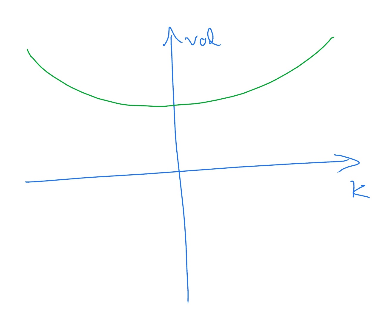
This picture is known as the volatility smile. The exact shape of the smile varies from market to market, and can also vary substantially over time. Sometimes the smile becomes inverted, and is known as a ‘volatility frown’.

The appearance of the volatility smile reflects deficiencies in the standard version of the Black-Scholes model. It is generally believed that the appearance of the volatility smile is closely connected to the standard Black-Scholes model not accounting for the possibility of jumps in the stock price; investigating this issue in detail is currently an active area of mathematical finance.

Despite the existence of the volatility smile, the Black-Scholes model is used extensively, in practice. The volatility smile provides an indicator of how well/badly the Black-Scholes model is capturing reality. It’s consequences, including what can be learned from the precise shape of the smile, are well understood by traders.

It should be noted that, in practice, decisions taken on trading stocks and shares are based both on information obtained using modelling techniques (such as Black-Scholes) as well as qualitative information (such as reading the annual general reports of companies, being aware of the political environment, etc). Combining all this information together is a difficult task, which requires understanding the modelling theory well enough to judge, in detail, which aspects of reality are modelled well and which are not. There is nothing special to the world of finance here – all sophisticated stochastic modelling requires this the same level of care.