Stochastic Processes and Financial Mathematics
(part two)

Chapter C Solutions to exercises (part two)

Chapter 11

11.1
- (a) We have $C_{t} = μ t + σ B_{t}$ . Hence,
  
  $\begin{aligned} E [C_{t}] & = E [μ t + σ B_{t}] = μ t + σ E [B_{t}] = μ t \\ E [C_{t}^{2}] & = E [μ^{2} t^{t} + 2 t μ σ B_{t} + σ^{2} B_{t}^{2}] = μ^{2} t^{2} + 2 t μ σ (0) + σ^{2} t = μ^{2} t^{2} + σ^{2} t \\ var (C_{t}) & = E [C_{t}^{2}] - E [C_{t}]^{2} = σ^{2} t . \end{aligned}$ where we use that $E [B_{t}] = 0$ and $E [B_{t}^{2}] = t$ .
- (b) We have
  
  $C_{t} - C_{u} = μ t + σ B_{t} - μ u - σ B_{u} = μ (t - u) + σ (B_{t} - B_{u}) \sim μ (t - u) + σ N (0, t - u)$
  
  where, in the final step, we use the definition of Brownian motion. Then, by the scaling properties normal random variables we have $C_{t} - C_{u} \sim N (μ (t - u), σ^{2} (t - u))$ .
- (c) Yes. By definition, Brownian motion $B_{t}$ is a continuous stochastic process, meaning that the probability that $B_{t}$ is a continuous function is one. Since $t \mapsto μ t$ is a continuous function, we have that $μ t + σ B_{t}$ is a continuous function with probability one; that is, $B_{t}$ is a continuous stochastic process.
- (d) We have $E [C_{t}] = μ t$ , but Brownian motion has expectation zero, so $C_{t}$ is not a Brownian motion.
11.2 We have

$\begin{aligned} cov (B_{u}, B_{t}) & = E [B_{t} B_{u}] - E [B_{t}] E [B_{u}] \\ = E [B_{t} B_{u}] \\ = E [(B_{t} - B_{u}) B_{u}] + E [B_{u}^{2}] \\ = E [B_{t} - B_{u}] E [B_{u}] + E [B_{u}^{2}] \\ = 0 \times 0 + u \\ = u \end{aligned}$ Here, to deduce the fourth line, we use the second property in Theorem 11.2.1, which tells us that $B_{t} - B_{u}$ and $B_{u}$ are independent.
11.3 When $u \leq t$ the martingale property of Brownian motion (Lemma 11.4.3) implies that $E [B_{t} | F_{u}] = B_{u}$ . When $t \leq u$ we have $B_{t} \in F_{u}$ so by taking out what is known we have $E [B_{t} | F_{u}] = B_{t}$ . Combing the two cases, for all $u \geq 0$ and $t \geq 0$ we have $E [B_{t} | F_{u}] = B_{min (u, t)}$ .
11.4
- (a) We’ll use the pdf of the normal distribution to write $E [B_{t}^{n}]$ as an integral. Then, integrating by parts (note that $\frac{d}{d z} e^{- \frac{z^{2}}{2 t}} = \frac{- z}{t} e^{- \frac{z^{2}}{2 t}}$ ) we have
  
  $\begin{aligned} E [B_{t}^{n}] & = \frac{1}{\sqrt{2 π t}} \int_{- \infty}^{\infty} z^{n} e^{- \frac{z^{2}}{2 t}} d z \\ = \frac{1}{\sqrt{2 π t}} \int_{- \infty}^{\infty} (- t z^{n - 1}) (\frac{- z}{t} e^{- \frac{z^{2}}{2 t}}) d z \\ = {[- \frac{1}{\sqrt{2 π t}} t z^{n - 1} e^{- \frac{z^{2}}{2 t}}]}_{z = - \infty}^{\infty} + \frac{1}{\sqrt{2 π t}} \int_{- \infty}^{\infty} t (n - 1) z^{n - 2} t e^{- \frac{z^{2}}{2 t}} d z \\ = 0 + t (n - 1) E [B_{t}^{n - 2}] . \end{aligned}$
- (b) We use the formula we deduced in part (a). Since $E [B_{t}^{0}] = E [1] = 1$ , we have $E [B_{t}^{2}] = t (2 - 1) (1) = t$ . Hence $E [B_{t}^{4}] = t (4 - 1) E [B_{t}^{2}] = t (4 - 1) t = 3 t^{2}$ and therefore $var (B_{t}^{2}) = E [B_{t}^{4}] - E [B_{t}^{2}]^{2} = 2 t^{2}$ .
- (c) Again, we use the formula we deduced in part (a). Since $E [B_{t}] = 0$ it follows (by a trivial induction) that $E [B_{t}^{n}] = 0$ for all odd $n \in N$ . For even $n \in N$ we have $E [B_{t}^{2}] = t$ and (by induction) we obtain
  
  $E [B_{t}^{n}] = t^{n / 2} (n - 1) (n - 3) \dots (1) .$
- (d) We have $var (B_{t}^{n}) = E [B_{t}^{2 n}] - E [B_{t}^{n}]^{2}$ which is finite by part (c). Hence $B_{t}^{n} \in L^{2}$ , which implies that $B_{t}^{n} \in L^{1}$ .
11.5 Using the scaling properties of normal random variables, we write $Z = μ + Y$ where $Y \sim N (0, σ^{2})$ . Then, $e^{Z} = e^{μ} e^{Y}$ and

$\begin{aligned} E [\exp (σ B_{t} - \frac{1}{2} σ^{2} t) | F_{u}] & = E [\exp (σ (B_{t} - B_{u}) + σ B_{u} - \frac{1}{2} σ^{2} t) | F_{u}] \\ = \exp (σ B_{u} - \frac{1}{2} σ^{2} t) E [\exp (σ (B_{t} - B_{u})) | F_{u}] \\ = \exp (σ B_{u} - \frac{1}{2} σ^{2} t) E [\exp (σ (B_{t} - B_{u}))] \\ = \exp (σ B_{u} - \frac{1}{2} σ^{2} t) \exp (\frac{1}{2} σ^{2} (t - u)) \\ = \exp (σ B_{u} - \frac{1}{2} σ^{2} u) . \end{aligned}$ Here, the second line follows by taking out what is known, since $B_{u}$ is $F_{u}$ measurable. The third line then follows by the definition of Brownian motion, in particular that $B_{t} - B_{u}$ is independent of $F_{u}$ . The fourth line follows by (11.2), since $B_{t} - B_{u} \sim N (0, t - u)$ and hence $σ (B_{t} - B_{u}) \sim N (0, σ^{2} (t - u))$ .
(b) Since $B_{t}$ is adapted, $B_{t}^{3} - 3 t B_{t}$ is also adapted. From 11.4 we have $B_{t}^{3}, B_{t} \in L^{1}$ , so also $B_{t}^{3} - t B_{t} \in L^{1}$ . Using that $B_{u}$ is $F_{u}$ measurable, we have

$\begin{aligned} E [B_{t}^{3} - 3 t B_{t} | F_{u}] & = E [(B_{u}^{3} - 3 u B_{u}) + B_{t}^{3} - 3 t B_{t} - (B_{u}^{3} - 3 u B_{u}) | F_{u}] \\ = B_{u}^{3} - 3 u B_{u} + E [B_{t}^{3} - B_{u}^{3} - 3 t B_{t} + 3 u B_{u} | F_{u}] \end{aligned}$ so we need only check that the second term on the right hand side is zero. To see this,

$\begin{aligned} E [B_{t}^{3} - B_{u}^{3} - 3 t B_{t} + 3 u B_{u} | F_{u}] & = E [B_{t}^{3} - B_{u}^{3} - 3 t B_{u} + 3 u B_{u} - 3 t (B_{t} - B_{u}) | F_{u}] \\ = E [B_{t}^{3} - B_{u}^{3} - 3 t B_{u} + 3 u B_{u} | F_{u}] + 0 \\ = E [B_{t}^{3} - B_{u}^{3} | F_{u}] - 3 B_{u} (t - u) \\ = E [(B_{t} - B_{u})^{3} + 3 B_{t}^{2} B_{u} - 3 B_{u}^{2} B_{t} | F_{u}] - 3 B_{u} (t - u) \\ = E [(B_{t} - B_{u})^{3} | F_{u}] + 3 B_{u} E [B_{t}^{2} | F_{u}] - 3 B_{u}^{2} E [B_{t} | F_{u}] - 3 B_{u} (t - u) \\ = E [(B_{t} - B_{u})^{3}] + 3 B_{u} (E [B_{t}^{2} - t | F_{u}] + t) - 3 B_{u}^{3} - 3 B_{u} (t - u) \\ = 0 + 3 B_{u} (B_{u}^{2} - u + t) - 3 B_{u}^{3} - 3 B_{u} (t - u) \\ = 0. \end{aligned}$ Here we use several applications of the fact that $B_{t} - B_{u}$ is independent of $F_{u}$ , whilst $B_{u}$ is $F_{u}$ measurable. We use also that $E [Z^{3}] = 0$ where $Z \sim N (0, σ^{2})$ , which comes from part (c) of 11.4 (or use that the normal distribution is symmetric about $0$ ), as well as that both $B_{t}$ and $B_{t}^{2} - t$ are martingales (from Lemmas 11.4.3 and 11.4.4).

11.7

(a) We have

$\begin{aligned} \sum_{k = 0}^{n - 1} (t_{k + 1} - t_{k}) & = (t_{n} - t_{n - 1}) + (t_{n - 1} - t_{n - 2}) + \dots + (t_{2} - t_{1}) + (t_{1} - t_{0}) \\ = t_{n} - t_{0} \\ = t - 0 \\ = t . \end{aligned}$ This is known as a ‘telescoping sum’. The same method shows that $\sum_{k = 0}^{n - 1} (B_{t_{k + 1}} - B_{t_{k}}) = B_{t} - B_{0} = 0$ .
(b) We need a bit more care for this one. We have

$\begin{aligned} 0 \leq \sum_{k = 0}^{n - 1} (t_{k + 1} - t_{k})^{2} & \leq \sum_{k = 0}^{n - 1} (t_{k + 1} - t_{k}) (max_{j = 0, \dots, n - 1} | t_{j + 1} - t_{j} |) \\ = (max_{j = 0, \dots, n - 1} | t_{j + 1} - t_{j} |) \sum_{k = 0}^{n - 1} (t_{k + 1} - t_{k}) \\ = (max_{j = 0, \dots, n - 1} | t_{j + 1} - t_{j} |) t . \end{aligned}$ Here, the last line is deduced using part (a). Letting $n \to 0$ we have $max_{j = 0, \dots, n - 1} | t_{j + 1} - t_{j} | \to 0$ , so the right hand side of the above tends to zero as $n \to \infty$ . Hence, using the sandwich rule, we have that $\sum_{k = 0}^{n - 1} (t_{k + 1} - t_{k})^{2} \to 0$ .
(c) Using the properties of Brownian motion, $B_{t_{k} + 1} - B_{t_{k}} \sim N (0, t_{k + 1} - t_{k})$ so from exercise 11.4 we have

$\begin{aligned} E [\sum_{k = 0}^{n - 1} (B_{t_{k} + 1} - B_{t_{k}})^{2}] & = \sum_{k = 0}^{n - 1} E [(B_{t_{k} + 1} - B_{t_{k}})^{2}] \\ = \sum_{k = 0}^{n - 1} (t_{k + 1} - t_{k}) \\ = t . \end{aligned}$ Here, the last line follows by part (a).

For the last part, the properties of Brownian motion give us that each increment $B_{t_{k + 1}} - B_{t_{k}}$ is independent of $F_{t_{k}}$ . In particular, the increments $B_{t_{k + 1}} - B_{t_{k}}$ are independent of each other. So, using exercise 11.4,

$\begin{aligned} var (\sum_{k = 0}^{n - 1} (B_{t_{k} + 1} - B_{t_{k}})^{2}) & = \sum_{k = 0}^{n - 1} var ((B_{t_{k} + 1} - B_{t_{k}})^{2}) \\ = \sum_{k = 0}^{n - 1} 2 (t_{k + 1} - t_{k})^{2} \end{aligned}$ which tends to zero as $n \to \infty$ , by the same calculation as in part (b).

11.8

(a) Let $y \geq 1$ . Then

$\begin{aligned} P [B_{t} \geq y] & = \int_{y}^{\infty} \frac{1}{\sqrt{2 π t}} e^{- \frac{z^{2}}{2 t}} d z \\ \leq \int_{y}^{\infty} \frac{1}{\sqrt{2 π t}} y e^{- \frac{z^{2}}{2 t}} d z \\ \leq \int_{y}^{\infty} \frac{1}{\sqrt{2 π t}} z e^{- \frac{z^{2}}{2 t}} d z \\ = \frac{1}{\sqrt{2 π t}} {[- t e^{- \frac{z^{2}}{2 t}}]}_{z = y}^{\infty} \\ = \sqrt{\frac{t}{2 π}} e^{- \frac{y^{2}}{2 t}} . \end{aligned}$ Putting $y = t^{α}$ where $α > \frac{1}{2}$ we have

$\begin{matrix} (C.1) & P [B_{t} \geq t^{α}] \leq \sqrt{\frac{t}{2 π}} e^{- \frac{1}{2} t^{2 α - 1}} . \end{matrix}$

Since $2 α - 1 \geq 0$ , the exponential term dominates the square root, and right hand side tends to zero as $t \to \infty$ .

If $α = \frac{1}{2}$ then we can use an easier method. Since $B_{t} \sim N (0, t)$ , we have $t^{- 1 / 2} B_{t} \sim N (0, 1)$ and hence

$P [B_{t} \geq t^{1 / 2}] = P [N (0, 1) \geq 1] \in (0, 1),$

which is independent of $t$ and hence does not tend to zero as $t \to \infty$ . Note that we can’t deduce this fact using the same method as for $α > \frac{1}{2}$ , because (C.1) only gives us an upper bound on $P [B_{t} \geq t^{α}]$ .
(b) For this we need a different technique. For $y \geq 0$ we integrate by parts to note that

$\begin{aligned} \int_{y}^{\infty} \frac{1}{\sqrt{2 π t}} e^{- \frac{- z^{2}}{2 t}} d z & = \frac{1}{\sqrt{2 π t}} \int_{y}^{\infty} \frac{1}{z} z e^{- \frac{- y^{2}}{2 t}} d z \\ = \frac{1}{\sqrt{2 π t}} ({[- \frac{t}{z} e^{- \frac{z^{2}}{2 t}}]}_{z = y}^{\infty} - \int_{y}^{\infty} \frac{t}{z^{2}} e^{- \frac{z^{2}}{2 t}}) d z \\ \leq \frac{1}{\sqrt{2 π t}} ({[- \frac{t}{z} e^{- \frac{z^{2}}{2 t}}]}_{z = y}^{\infty}) \\ = \frac{1}{\sqrt{2 π t}} \frac{t}{y} e^{- \frac{y^{2}}{2 t}} \\ = \frac{t}{\sqrt{2 π}} \frac{1}{y} e^{- \frac{y^{2}}{2 t}} \end{aligned}$ Using the symmetry of normal random variables about $0$ , along with this inequality, we have

$\begin{aligned} P [| B_{t} | \geq a] & = P [B_{t} \geq a] + P [B_{t} \leq - a] \\ = 2 P [B_{t} \geq a] \\ \leq 2 \frac{t}{\sqrt{2 π}} \frac{1}{a} e^{- \frac{a^{2}}{2 t}} . \end{aligned}$ As $t ↘ 0$ , the exponential term tends to $0$ , which dominates the $\sqrt{t}$ , meaning that $P [| B_{t} | \geq a] \to 0$ as $t ↘ 0$ . That is, $B_{t} \to 0$ in probability as $t ↘ 0$ .

Chapter 12

12.1 From (12.8) we have both $\int_{0}^{t} 1 d B_{u} = B_{t}$ and $\int_{0}^{s} d B_{u} = B_{s}$ , and using (12.6) we obtain

$\int_{u}^{t} 1 d B_{u} = \int_{0}^{t} 1 d B_{u} - \int_{0}^{v} 1 d B_{u} = B_{t} - B_{v} .$
12.2 Since $B_{t}$ is adapted to $F_{t}$ , we have that $e^{B_{t}}$ is adapted to $F_{t}$ . Since $B_{t}$ is a continuous stochastic process and $\exp (\cdot)$ is a continuous function, $e^{B_{t}}$ is also continuous. From (11.2) we have that

$\begin{aligned} \int_{0}^{t} E [{(e^{B_{u}})}^{2}] d u & = \int_{0}^{t} E [e^{2 B_{u}}] d u \\ = \int_{0}^{t} e^{\frac{1}{2} (2^{2}) u} d u \\ = \int_{0}^{t} e^{2 u} d u < \infty . \end{aligned}$ Therefore, $e^{B_{t}} \in H^{2}$ .
12.3
- (a) We have
  
  $E [e^{\frac{Z^{2}}{2}}] = \frac{1}{\sqrt{2 π}} \int_{- \infty}^{\infty} e^{\frac{z^{2}}{2}} e^{\frac{- z^{2}}{2}} d z = \frac{1}{\sqrt{2 π}} \int_{- \infty}^{\infty} 1 d z = \infty .$
- (b) Using the scaling properties of normal distributions, $t^{- 1 / 2} B_{t}$ has a $N (0, 1)$ distribution for all $t$ . Hence, if we set $F_{t} = t^{- 1 / 2} B_{t}$ then by part (a) we have
  
  $\int_{0}^{t} E [e^{\frac{1}{2} F_{t}^{2}}] d u = \int_{0}^{t} \infty d u$
  
  which is not finite. Note also that $F_{t}$ is adapted to $F_{t}$ . Since $e^{t}$ , $t^{2}$ , $t^{- 1 / 2}$ and $B_{t}$ are all continuous, so is $e^{\frac{1}{2} F_{t}^{2}}$ . Hence $e^{\frac{1}{2} F_{t}^{2}}$ is an example of a continuous, adapted stochastic process that is not in $H^{2}$ .
  
  Note that we can’t simply use the stochastic process $F_{t} = Z$ , because we have nothing to tell us that $Z$ is $F_{t}$ measurable.
12.4 We have

$\begin{aligned} E [X_{t}] & = E [2] + E [\int_{0}^{t} t + B_{u}^{2} d u] + E [\int_{0}^{t} B_{u}^{2} d B_{u}] \\ = 2 + \int_{0}^{t} t + E [B_{u}^{2}] d u + 0 \\ = 2 + t^{2} + \int_{0}^{t} u d u \\ = 2 + t^{2} + \frac{t^{2}}{2} \\ = 2 + \frac{3 t^{2}}{2} . \end{aligned}$
12.5
- (a) $X_{t} = 0 + \int_{0}^{t} 0 d u + \int_{0}^{t} 0 d B_{u}$ so $X_{t}$ is an Ito process.
- (b) $Y_{t} = 0 + \int_{0}^{t} 2 u d u + \int_{0}^{t} 1 d B_{u}$ by (12.8), so $Y_{t}$ is an Ito process.
- (c) A symmetric random walk is a process in discrete time, and is therefore not an Ito process.
12.6 We have

$\begin{aligned} E [V_{t}] & = E [e^{- k t} v] + σ e^{- k t} E [\int_{0}^{t} e^{k s} d B_{s}] \\ = e^{- k t} v . \end{aligned}$ Here we use Theorem 12.2.1 to show that the expectation of the $d B_{u}$ integral is zero. In order to calculate $var (V_{t})$ we first calculate

$\begin{aligned} E [V_{t}^{2}] & = E [e^{- 2 k t} v^{2}] + 2 σ e^{- k t} E [\int_{0}^{t} e^{k s} d B_{s}] + σ^{2} e^{- 2 k t} E [{(\int_{0}^{t} e^{k s} d B_{s})}^{2}] \\ = e^{- 2 k t} v^{2} + 0 + σ^{2} e^{- 2 k t} \int_{0}^{t} E [(e^{k s})^{2}] d u \\ = e^{- 2 k t} v^{2} + σ^{2} e^{- 2 k t} \int_{0}^{t} e^{2 k u} d u \\ = e^{- 2 k t} v^{2} + σ^{2} e^{- 2 k t} \frac{1}{2 k} (e^{2 k t} - 1) \\ = e^{- 2 k t} v^{2} + \frac{σ^{2}}{2 k} (1 - e^{- 2 k t}) \end{aligned}$ Again, we use Theorem 12.2.1 to calculate the final term on the first line. We obtain that

$\begin{aligned} var (V_{t}) & = E [V_{t}^{2}] - E [V_{t}]^{2} \\ = \frac{σ^{2}}{2 k} (1 - e^{- 2 k t}) . \end{aligned}$
12.7 We have

$X_{t} = μ t + \int_{0}^{t} σ_{u} d B_{u} .$

Since $M_{t} = \int_{0}^{t} σ_{u} d B_{u}$ is a martingale (by Theorem 12.2.1), we have that $M_{t}$ is adapted and in $L^{1}$ , and hence also $X_{t}$ is adapted and in $L^{1}$ . For $v \leq t$ we have

$\begin{aligned} E [X_{t} | F_{v}] & = μ t + E [M_{t} | F_{v}] \\ = μ t + M_{v} \\ = μ t + \int_{0}^{v} σ_{u} d B_{u} \\ \geq μ v + \int_{0}^{v} σ_{u} d B_{u} \\ = X_{v} . \end{aligned}$ Hence, $X_{t}$ is a submartingale.
12.8
- (a) Taking $F_{t} = 0$ , we have $E [F_{t}] =$ and $\int_{0}^{t} F_{s} d s = 0$ , hence $\int_{0}^{t} E [F_{s}] d s = E [\int_{0}^{t} F_{s} d B_{s}] = 0$ .
- (b) Taking $F_{t} = 1$ , we have $E [F_{t}] = 1$ and $\int_{0}^{t} F_{s} d s = t$ , hence $\int_{0}^{t} E [F_{s}] d s = t$ and $E [\int_{0}^{t} F_{s} d B_{s}] = E [B_{t}] = 0$ .
12.9
- (a) We have $(| X | - | Y |)^{2} \geq 0$ , so $2 | X Y | \leq X^{2} + Y^{2}$ , which by monotonicity of $E$ means that $2 E [| X Y |] \leq E [X^{2}] + E [Y^{2}]$ . Using the relationship between $E$ and $| \cdot |$ we have
  
  $2 | E [X Y] | \leq 2 E [| X Y |] \leq E [X^{2}] + E [Y^{2}] .$
- (b) Let $X_{t}, Y_{t} \in H^{2}$ and let $α, β \in R$ be deterministic constants. We need to show that $Z_{t} α X_{t} + β Y_{t} \in H^{2}$ . Since both $X_{t}$ and $Y_{t}$ are continuous and adapted, $Z_{t}$ is also both continuous and adapted. It remains to show that (12.5) holds for $Z_{t}$ . With this in mind we note that
  
  $Z_{t}^{2} = α^{2} X_{t}^{2} + 2 α β X_{t} Y_{t} + β^{2} Y_{t}^{2}$
  
  and hence that
  
  $\begin{aligned} | E [Z_{t}^{2}] | & = | α^{2} E [X_{t}^{2}] + 2 α β E [X_{t} Y_{t}] + β^{2} E [Y_{t}^{2}] | \\ \leq α^{2} E [X_{t}^{2}] + 2 | α β | | E [X_{t} Y_{t}] | + β^{2} E [Y_{t}^{2}] \\ \leq α^{2} E [X_{t}^{2}] + | α β | (E [X_{t}^{2}] + E [Y_{t}^{2}]) + β^{2} E [Y_{t}^{2}] \\ = (α^{2} + | α β |) E [X_{t}^{2}] + (β^{2} + | α β |) | E [Y_{t}^{2}] . \end{aligned}$ where we use part (a) to deduce the third line from the second. Hence,
  
  $\begin{aligned} \int_{0}^{t} E [Z_{u}^{2}] d u & \leq \int_{0}^{t} (α^{2} + | α β |) E [X_{u}^{2}] + (β^{2} + | α β |) | E [Y_{u}^{2}] d u \\ = (α^{2} + | α β |) \int_{0}^{t} E [X_{u}^{2}] d u + (β^{2} + | α β |) \int_{0}^{t} E [Y_{u}^{2}] d u < \infty \end{aligned}$ as required. The final line is $< \infty$ because $X_{t}, Y_{t} \in H^{2}$ .
12.10 We have $I_{F} (t) = \sum_{i = 1}^{n} F_{t_{i - 1}} [B_{t_{i} \land t} - B_{t_{i - 1} \land t}] .$ We are looking to show that

$\begin{matrix} (C.2) & E [I_{F} (t)^{2}] = \int_{0}^{t} E [F_{u}^{2}] d u . \end{matrix}$

On the right hand side we have

$\begin{aligned} \int_{0}^{t} E [F_{u}^{2}] d u & = \sum_{i = 1}^{m} \int_{t_{i - 1 \land t}}^{t_{i} \land t} E [F_{u}^{2}] d u \\ (C.3) & = \sum_{i = 1}^{m} (t_{i} \land t - t_{i - 1} \land t) E [F_{t_{i - 1}}^{2}] \end{aligned}$ because $F_{t}$ is constant during each time interval $[t_{i - 1} \land t, t_{i} \land t)$ . On the left hand side of (C.2) we have

$\begin{aligned} E [I_{F} (t)^{2}] & = E [{(\sum_{i = 1}^{m} F_{t_{i - 1}} [B_{t_{i} \land t} - B_{t_{i - 1} \land t}])}^{2}] \\ = E [\sum_{i = 1}^{m} F_{t_{i - 1}}^{2} [B_{t_{i} \land t} - B_{t_{i - 1} \land t}]^{2} + 2 \sum_{i = 1}^{m} \sum_{j = 1}^{i - 1} F_{t_{i - 1}} F_{t_{j - 1}} [B_{t_{i} \land t} - B_{t_{i - 1} \land t}] [B_{t_{j} \land t} - B_{t_{j - 1} \land t}]] \\ = \sum_{i = 1}^{m} E [F_{t_{i - 1}}^{2} [B_{t_{i} \land t} - B_{t_{i - 1} \land t}]^{2}] + 2 \sum_{i = 1}^{m} \sum_{j = 1}^{i - 1} E [F_{t_{i - 1}} F_{t_{j - 1}} [B_{t_{i} \land t} - B_{t_{i - 1} \land t}] [B_{t_{j} \land t} - B_{t_{j - 1} \land t}]] \end{aligned}$ In the first sum, using the tower rule, taking out what is known, independence, and then the fact that $E [B_{t}^{2}] = t$ , we have

$\begin{aligned} E [F_{t_{i - 1}}^{2} [B_{t_{i} \land t} - B_{t_{i - 1} \land t}]^{2}] & = E [E [F_{t_{i - 1}}^{2} [B_{t_{i} \land t} - B_{t_{i - 1} \land t}]^{2} | F_{t_{i - 1}}]] \\ = E [F_{t_{i - 1}}^{2} E [[B_{t_{i} \land t} - B_{t_{i - 1} \land t}]^{2} | F_{t_{i - 1}}]] \\ = E [F_{t_{i - 1}}^{2} E [[B_{t_{i} \land t} - B_{t_{i - 1} \land t}]^{2}]] \\ = E [F_{t_{i - 1}}^{2} (t_{i} \land t - t_{i - 1} \land t)] \end{aligned}$ In the second sum, since $j < i$ we have $t_{j - 1} \leq t_{i}$ , so using the tower rule, taking out what is known, and then the martingale property of Brownian motion, we have

$\begin{aligned} E [F_{t_{i - 1}} F_{t_{j - 1}} [B_{t_{i} \land t} - B_{t_{i - 1} \land t}] [B_{t_{j} \land t} - B_{t_{j - 1} \land t}]] & = E [E [F_{t_{i - 1}} F_{t_{j - 1}} [B_{t_{i} \land t} - B_{t_{i - 1} \land t}] [B_{t_{j} \land t} - B_{t_{j - 1} \land t}] | F_{t_{i - 1}}]] \\ = E [F_{t_{j - 1}} [B_{t_{j} \land t} - B_{t_{j - 1} \land t}] F_{t_{i - 1}} (E [B_{t_{i} \land t} | F_{t_{i - 1}}] - B_{t_{i - 1} \land t})] \\ = E [F_{t_{j - 1}} [B_{t_{j} \land t} - B_{t_{j - 1} \land t}] F_{t_{i - 1}} (B_{t_{i - 1} \land t} - B_{t_{i - 1} \land t})] \\ = 0. \end{aligned}$ Therefore,

$E [I_{F} (t)^{2}] = \sum_{i = 1}^{m} E [F_{t_{i - 1}}^{2} (t_{i} \land t - t_{i - 1} \land t)]$

which matches (C.3) and completes the proof.

Chapter 13

13.1
- (a) $X_{t} = X_{0} + \int_{0}^{t} 2 u d u + \int_{0}^{t} B_{u} d B_{u}$ .
- (b) $Y_{T} = Y_{t} + \int_{t}^{T} u d u$ .
By using the fundamental theorem of calculus, we obtain that $Y$ satisfies the differential equation $\frac{d Y_{t}}{d t} = t$ . Using equation (13.6) from Example 13.1.2, we have that

$\begin{array}{r} X_{t} = X_{0} + t^{2} + \frac{B_{t}^{2}}{2} - \frac{t}{2} \end{array}$ which is not differentiable because $B_{t}$ is not differentiable.
13.2 We have $Z_{t} = f (t, X_{t})$ where $f (t, x) = t^{3} x$ and $d X_{t} = α d t + β d B_{t}$ . By Ito’s formula,

$\begin{aligned} \frac{n (n - 1)}{2} \int_{0}^{t} u^{(n - 2) / 2} (n - 3) (n - 5) \dots (1) d u & = \frac{n (n - 1)}{2} \frac{t^{n / 2}}{n / 2} (n - 3) (n - 5) \dots (1) d u \\ = t^{n / 2} (n - 1) (n - 3) \dots (1) \end{aligned}$ as required.
13.5
- (a) By Ito’s formula, with $f (t, x) = e^{t / 2} \cos x$ , we have
  
  $\begin{aligned} d X_{t} & = (\frac{1}{2} e^{t / 2} \cos (B_{t}) + (0) (- e^{t / 2} \sin (B_{t})) + \frac{1}{2} (1^{2}) (- e^{t / 2} \cos (B_{t}))) d t + (1) (- e^{t / 2} \sin (B_{t})) d B_{t} \\ = - e^{t / 2} \sin (B_{t}) d B_{t} . \end{aligned}$ Hence $X_{t} = X_{0} - \int_{0}^{t} e^{u / 2} \sin (B_{u}) d B_{u}$ , which is martingale by Theorem 12.2.1.
- (b) By Ito’s formula, with $f (t, x) = (x + t) e^{- x - t / 2}$ we have
  
  $\begin{aligned} d Y_{t} & = {e^{- B_{t} - t / 2} - \frac{1}{2} (B_{t} + t) e^{- B_{t} - t / 2} + (0) (e^{- B_{t} - t / 2} - (B_{t} + t) e^{- B_{t} - t / 2}) \\ + \frac{1}{2} (1^{2}) (- e^{- B_{t} - t / 2} - e^{- B_{t} - t / 2} + (B_{t} + t) e^{- B_{t} - t / 2})} d t \\ + (1^{2}) (e^{- B_{t} - t / 2} - (B_{t} + t) e^{- B_{t} - t / 2}) d B_{t} \\ = (1 - t - B_{t}) e^{- B_{t} - t / 2} d B_{t} . \end{aligned}$ Hence $Y_{t} = Y_{0} + \int_{0}^{t} (1 - u - B_{u}) e^{- B_{u} - u / 2} d B_{u}$ , which is martingale by Theorem 12.2.1.
13.6 We apply Ito’s formula with $f (t, x) = t x$ to $Z_{t} = f (t, B_{t}) = t B_{t}$ and obtain

$d Z_{t} = (B_{t} + (0) (t) + \frac{1}{2} (1^{2}) (0)) d t + (1) (t) d B_{t}$

so we obtain

$t B_{t} = 0 B_{0} + \int_{0}^{t} B_{u} d u + \int_{0}^{t} u d B_{u},$

as required.
13.7
- (a) We have $X_{t} = X_{0} + \int_{0}^{t} 2 + 2 s d s + \int_{0}^{t} B_{s} d B_{s}$ . Taking expectations, and recalling that Ito integrals have zero mean, we obtain that
  
  $E [X_{t}] = X_{0} + \int_{0}^{t} 2 + 2 s d s + 0 = 1 + {[2 s + s^{2}]}_{s = 0}^{t} = 1 + 2 t + t^{2} = (1 + t)^{2} .$
- (b) From Ito’s formula,
  
  $\begin{aligned} d Y_{t} & = (0 + (2 + 2 t) (2 X_{t}) + \frac{1}{2} (B_{t})^{2} (2)) d t + B_{t} (2 X_{t}) d B_{t} \\ = (4 (1 + t) X_{t} + (B_{t})^{2}) d t + 2 X_{t} B_{t} d B_{t} . \end{aligned}$ Writing in integral form, taking expectations, and using that Ito integrals have zero mean, we obtain
  
  $\begin{aligned} E [Y_{t}] & = Y_{0} + E [\int_{0}^{t} 4 (1 + s) X_{t} + (B_{s})^{2} d s] + 0 \\ = 1 + \int_{0}^{t} 4 (1 + s) E [X_{s}] + E [B_{s}^{2}] d s \\ = 1 + \int_{0}^{t} 4 (1 + s)^{3} + s d s \\ = 1 + {[(1 + s)^{4} + \frac{s^{2}}{2}]}_{s = 0}^{t} \\ = (1 + t)^{4} + \frac{t^{2}}{2} \end{aligned}$ Hence, using that $E [X_{t}^{2}] = E [Y_{t}]$ ,
  
  $\begin{aligned} var (X) & = E [X_{t}^{2}] - E [X_{t}]^{2} \\ = (1 + t)^{4} + \frac{t^{2}}{2} - (1 + t)^{4} \\ = \frac{t^{2}}{2} . \end{aligned}$
- (c) If we change the $d B_{t}$ coefficient then we won’t change the mean, because we can see from (a) that $E [X_{t}]$ depends only on the $d B_{t}$ coefficient. However, as we can see from part (b), the variance depends on both the $d t$ and $d B_{t}$ terms, so will typically change if we alter the $d B_{t}$ coefficient.
13.8 In integral form, we have

$X_{t} = X_{0} + \int_{0}^{t} α X_{u} d u + \int_{0}^{t} σ_{u} d B_{u} .$

Taking expectations, swapping $\int d u$ with $E$ , and recalling from Theorem 12.2.1 that Ito integrals are zero mean martingales, we obtain

$E [X_{t}] = E [X_{0}] + \int_{0}^{t} α E [X_{u}] d u .$

Applying the fundamental theorem of calculus, if we set $x_{t} = E [X_{t}]$ , we obtain

$\frac{d x_{t}}{d t} = α x_{t}$

which has solution $x_{t} = C e^{α t}$ . Putting in $t = 0$ shows that $C = E [X_{0}] = 1$ , hence

$E [X_{t}] = e^{α t} .$
13.9 We have $X_{t} = X_{0} + \int_{0}^{t} X_{s} d B_{s}$ . Since Ito integrals are zero mean martingales, this means that $E [X_{t}] = E [X_{0}] = 1$ . Writing $Y_{t} = X_{t}^{2}$ and using Ito’s formula,

$\begin{aligned} d Y_{t} & = (0 + (0) (2 X_{t}) + \frac{1}{2} (X_{t})^{2} (2)) d t + (X_{t}) (2 X_{t}) d B_{t} \\ = (X_{t}^{2}) d t + 2 X_{t}^{2} d B_{t} . \\ = Y_{t} d t + 2 Y_{t} d B_{t} \end{aligned}$ Writing in integral form and taking expectations, we obtain

$\begin{aligned} E [Y_{t}] & = 1 + \int_{0}^{t} E [Y_{s}] d s + 0. \end{aligned}$ Hence, by the fundamental theorem of calculus, $f (t) = E [Y_{t}]$ satisfies the differential equation $f^{'} (t) = f (t)$ . The solution of this differential equation is $f (t) = A e^{t}$ . Since $E [Y_{0}] = 1$ we have $A = 1$ and thus $E [Y_{t}] = e^{t}$ . Hence,

$var (X_{t}) = E [X_{t}^{2}] - E [X_{t}]^{2} = E [Y_{t}] - 1 = e^{t} - 1.$
13.10

Recall that $cov (X_{s}, X_{t}) = E [(X_{t} - E [X_{t}]) (X_{s} - E [X_{s}])$ . From (13.12) we have

$E [X_{t}] = E [e^{- θ t} (X_{t} - μ)] + E [\int_{0}^{t} e^{- θ (t - u)} d B_{u}] = E [e^{- θ t} (X_{t} - μ)] + 0,$

because Ito integrals are zero mean martingales. Thus $X_{t} - E [X_{t}] = \int_{0}^{t} σ e^{θ (u - t)} d B_{u}$ . We can now calculate

$\begin{aligned} cov (X_{s}, X_{t}) & = Cov (\int_{0}^{s} σ e^{θ (u - s)} d B_{u}, \int_{0}^{t} σ e^{θ (v - t)} d B_{v}) \\ = E [(\int_{0}^{s} σ e^{θ (u - s)} d B_{u}) (\int_{0}^{t} σ e^{θ (v - t)} d B_{v})] \\ = σ^{2} e^{- θ (s + t)} E [(\int_{0}^{s} e^{θ u} d B_{u}) (\int_{0}^{t} e^{θ v} d B_{v})] \\ = σ^{2} e^{- θ (s + t)} E [(\int_{0}^{s} e^{θ u} d B_{u} + \int_{s}^{t} e^{θ u} d B_{u}) (\int_{0}^{s} e^{θ v} d B_{v})] \\ = σ^{2} e^{- θ (s + t)} E [(\int_{0}^{s} e^{θ u} d B_{u})^{2}] + E [(\int_{0}^{s} e^{θ v} d B_{v}) (\int_{s}^{t} e^{θ u} d B_{u})] \\ = σ^{2} e^{- θ (s + t)} \int_{0}^{s} e^{2 θ u} d u + E [\int_{0}^{s} e^{θ v} d B_{v}] E [\int_{s}^{t} e^{θ u} d B_{u}] \\ = \frac{σ^{2}}{2 θ} e^{- θ (s + t)} (e^{2 θ s} - 1) + 0. \end{aligned}$ In the above, the second line and final lines follow because Ito integrals have zero mean. The penultimate line follows because $\int_{0}^{s} e^{θ v} d B_{v}$ and $\int_{s}^{t} e^{θ u} d B_{u}$ are independent. This fact follows from the independence property in Theorem 11.2.1 (which defines Brownian motion), which implies that $σ (B_{v} - B_{u}; v \geq u \geq s)$ and $σ (B_{v} - B_{u}; s \geq v \geq u)$ are independent. Note that from (12.3) we know that $\int_{a}^{b} F_{u} d B_{s}$ only depends on increments of Brownian motion between times $a$ and $b$ . (The same fact can be deduced from the Markov property from Section 14.2.)

Hence $var (X_{t}) = \frac{σ^{2}}{2 θ} e^{- θ (2 t)} (e^{2 θ t} - 1) = \frac{σ^{2}}{2 θ} (1 - e^{- 2 θ t})$ . It follows immediately that $var (X_{t}) \to \frac{σ^{2}}{2 θ}$ as $t \to \infty$ .
13.11
- (a) Applying Ito’s formula to $Z_{t} = B_{t}^{3}$ , with $f (t, x) = x^{3}$ , we have
  
  $\begin{aligned} d Z_{t} & = (0 + (0) (3 B_{t}^{2}) + \frac{1}{2} (1^{2}) (6 B_{t})) d t + (1) (3 B_{t}^{2}) d B_{t} \\ = 3 B_{t} d t + 3 B_{t}^{2} d t \end{aligned}$ and substituting in for $Z$ we obtain
  
  $d Z_{t} = 3 Z_{t}^{1 / 3} d t + 3 Z_{t}^{2 / 3} d B_{t}$
  
  as required.
- (b) Another solution is the (constant, deterministic) solution $X_{t} = 0$ .
13.12 Equation (13.9) says that

$X_{t} = X_{0} \exp ((α - \frac{1}{2} σ^{2}) t + σ B_{t}) .$

Using Ito’s formula, with $f (t, x) = X_{0} \exp ((α - \frac{1}{2} σ^{2}) t + σ x)$ we obtain

$\begin{aligned} d X_{t} & = ((α - \frac{1}{2} σ^{2}) X_{t} + (0) (σ X_{t}) + \frac{1}{2} (1^{2}) (σ^{2} X_{t})) d t + (1) (σ X_{t}) d B_{t} \\ = α X_{t} d t + σ X_{t} d B_{t} \end{aligned}$ and thus $X_{t}$ solves (13.8).
13.13 Equation (13.14) says that

$X_{t} = X_{0} \exp (\int_{0}^{t} σ_{u} d B_{u} - \frac{1}{2} \int_{0}^{t} σ_{u}^{2} d u)$

We need to arrange this into a form where we can apply Ito’s formula. We write

$X_{t} = X_{0} \exp (Y_{t} - \frac{1}{2} \int_{0}^{t} σ_{u}^{2} d u)$

where $d Y_{t} = σ_{t} d B_{t}$ with $Y_{0} = 0$ . We now have $X_{t} = f (t, Y_{t})$ where $f (t, y) = X_{0} \exp (y - \frac{1}{2} \int_{0}^{t} σ_{u} d u)$ , so from Ito’s formula (and the fundamental theorem of calculus) we obtain

$\begin{aligned} d X_{t} & = (- \frac{1}{2} σ_{t}^{2} X_{t} + (0) (X_{t}) + \frac{1}{2} (σ_{t}^{2}) (X_{t})) d t + (σ_{t}) (X_{t}) d B_{t} \\ = σ_{t} X_{t} d B_{t} . \end{aligned}$ Hence, $X_{t}$ solves (13.13).
13.14
- (a) This is essentially Example 3.3.9 but in continuous time. By definition of conditional expectation (i.e. Theorem 3.1.1) we have that $M_{t} \in L^{1}$ and that $M_{t} \in F_{t}$ . It remains only to use the tower property to note that for $0 \leq u \leq t$ we have
  
  $E [M_{t} | F_{u}] = E [E [Y | F_{t}] F_{u}] = E [Y | F_{u}] = M_{u} .$
- (b)
  - (i) Note that $M_{0} = E [B_{T}^{2} | F_{0}] = E [B_{T}^{2}] = T$ . We showed in Lemma 11.4.4 that $B_{t}^{2} - t$ was a martingale, hence
    
    $\begin{aligned} E [B_{T}^{2} | F_{t}] & = E [B_{T}^{2} - T + T | F_{t}] \\ = B_{t}^{2} - t + T \end{aligned}$ Using (13.6), this gives us that
    
    $E [B_{T}^{2} | F_{t}] = 2 \int_{0}^{t} B_{u} d B_{u} + t - t + T$
    
    so we obtain
    
    $M_{t} = T + \int_{0}^{t} 2 B_{u} d B_{u}$
    
    and we can take $h_{t} = 2 B_{t}$ .
  - (ii) Note that $M_{0} = E [B_{T}^{3} | F_{0}] = E [B_{T}^{3}] = 0$ . We showed in 11.6 that $B_{t}^{3} - 3 t B - t$ was a martingale. Hence,
    
    $\begin{aligned} E [B_{T}^{3} | F_{t}] & = E [B_{T}^{3} - 3 T B_{T} + 3 T B_{T} | F_{t}] \\ = B_{t}^{3} - 3 t B_{t} + 3 T B_{t} . \end{aligned}$ Using Ito’s formula on $Z_{t} = B_{t}^{3}$ , we obtain $d Z_{t} = {0 + (0) (3 B_{t}^{2}) + \frac{1}{2} (1^{2}) (6 B_{t})} d t + (1) (3 B_{t}^{2}) d B_{t}$ so as
    
    $B_{t}^{3} = 0 + \int_{0}^{t} 3 B_{u} d u + \int_{0}^{t} 3 B_{u}^{2} d B_{u} .$
    
    Also, from 13.6 we have
    
    $t B_{t} = \int_{0}^{t} B_{u} d u + \int_{0}^{t} u d B_{u},$
    
    so as
    
    $\begin{aligned} E [B_{T}^{3} | F_{t}] & = 3 \int_{0}^{t} B_{u} d u + 3 \int_{0}^{t} B_{u}^{2} d B_{u} - 3 (\int_{0}^{t} B_{u} d u + \int_{0}^{t} u d B_{u}) + 3 T B_{t} \\ = 3 \int_{0}^{t} B_{u}^{2} d B_{u} - 3 \int_{0}^{t} u d B_{u} + 3 T \int_{0}^{t} 1 d B_{u} \\ = \int_{0}^{t} 3 B_{u}^{2} - 3 u + 3 T d B_{u} . \end{aligned}$ We can take $h_{t} = 3 B_{t}^{2} - 3 t + 3 T$ .
  - (iii) Note that $M_{0} = E [e^{σ B_{T}} | F_{0}] = E [e^{σ B_{T}}] = e^{\frac{1}{2} σ^{2} T}$ by (11.2) and the scaling properties of normal random variables. We showed in 11.6 that $e^{σ B_{t} - \frac{1}{2} σ^{2} t}$ was a martingale. Hence,
    
    $\begin{aligned} E [e^{σ B_{T}} | F_{t}] & = E [e^{σ B_{T} - \frac{1}{2} σ^{2} T} e^{\frac{1}{2} σ^{2} T} | F_{t}] \\ = e^{σ B_{t} - \frac{1}{2} σ^{2} t} e^{\frac{1}{2} σ^{2} T} \\ = e^{σ B_{t} - \frac{1}{2} σ^{2} (T - t)} . \end{aligned}$ Applying Ito’s formula to $Z_{t} = e^{σ B_{t} - \frac{1}{2} σ^{2} (T - t)}$ gives that
    
    $\begin{aligned} d Z_{t} & = (- \frac{1}{2} σ^{2} Z_{t} + (0) (σ Z_{t}) + \frac{1}{2} (1^{2}) (σ^{2} Z_{t})) d t + (1) (σ Z_{t}) d B_{t} \\ = σ Z_{t} d B_{t} \end{aligned}$ so we obtain that
    
    $Z_{t} = Z_{0} + \int_{0}^{t} σ Z_{u} d B_{u} .$
    
    Substituting in for $Z_{t}$ we obtain
    
    $E [e^{σ B_{T}} | F_{t}] = e^{\frac{1}{2} σ^{2} T} + \int_{0}^{t} σ Z_{u} d B_{u}$
    
    so we can take $h_{t} = σ Z_{t} = σ e^{σ B_{t} - \frac{1}{2} σ^{2} (T - t)}$ .

Chapter 14

14.1 We have $α (t, x) = - 2 t$ , $β = 0$ and $Φ (x) = e^{x}$ . By Lemma 14.1.2 the solution is given by

$F (t, x) = E_{t, x} [e^{X_{T}}]$

where $d X_{u} = - 2 u d u + 0 d B_{u} = d u$ . This gives

$\begin{aligned} X_{T} & = X_{t} - \int_{t}^{T} 2 u d u \\ = X_{t} - T^{2} + t^{2} . \end{aligned}$ Hence,

$\begin{aligned} F (t, x) & = E_{t, x} [e^{X_{t} - t^{2}}] \\ = E [e^{x - T^{2} + t^{2}}] \\ = e^{x} e^{- T^{2} + t^{2}} . \end{aligned}$ Here we use that $X_{t} = x$ under $E_{t, x}$ .
14.2 We have $α = β = 1$ and $Φ (x) = x^{2}$ . By Lemma 14.1.2 the solution is given by

$F (t, x) = E_{t, x} [X_{T}^{2}]$

where $d X_{u} = d u + d B_{u}$ . This gives

$\begin{aligned} X_{T} & = X_{t} + \int_{t}^{T} d u + \int_{t}^{T} d B_{u} \\ = X_{t} + (T - t) + (B_{T} - B_{t}) . \end{aligned}$ Hence,

$\begin{aligned} F (t, x) & = E_{t, x} [{(X_{t} + (T - t) + (B_{T} - B_{t}))}^{2}] \\ = E [x^{2} + (T - t)^{2} + (B_{T} - B_{t})^{2} + 2 x (T - t) + 2 x (B_{T} - B_{t}) + 2 (T - t) (B_{T} - B_{t})] \\ = x^{2} + (T - t)^{2} + (T - t) + 2 x (T - t) . \end{aligned}$ Here we use that $X_{t} = x$ under $E_{t, x}$ and that $B_{T} - B_{t} \sim B_{T - t} \sim N (0, T - t) .$
14.3
- (a) We have $Z_{t} = F (t, X_{t}) + γ (t)$ , where $d X_{t} = α (t, x) d t + β (t, x) d B_{t}$ , so
  
  $\begin{aligned} d Z_{t} & = (\frac{\partial F}{\partial t} + \frac{\partial γ}{\partial t} (t) + α (t, x) \frac{\partial F}{\partial x} + \frac{1}{2} β (t, x)^{2} \frac{\partial^{2} F}{\partial x^{2}}) d t + β (t, x) \frac{\partial F}{\partial x} d B_{t} \\ = β (t, x) \frac{\partial F}{\partial x} d B_{t} \end{aligned}$ where as usual we have suppressed the $(t, X_{t})$ arguments of $F$ and its partial derivatives. Note that the term in front of the $d t$ is zero because $F$ satisfies (14.8).
- (b) We use the same strategy as in the proof of Lemma 14.1.2. Writing out $d Z_{t}$ in integral form over time interval $[t, T]$ we obtain
  
  $Z_{T} = Z_{t} + \int_{t}^{T} β (u, x) \frac{\partial F}{\partial x} d B_{u} .$
  
  Taking expectations $E_{t, x}$ gives us
  
  $E_{t, x} [F (T, X_{T}) + γ (T)] = E_{t, x} [F (t, X_{t}) + γ (t)]$
  
  and noting that $X_{t} = x$ under $E_{t, x}$ , we have
  
  $E_{x, t} [F (T, X_{T})] + γ (T) = F (t, x) + γ (t) .$
  
  Using (14.9) we have $F (T, X_{T}) = Φ (X_{T})$ and we obtain
  
  $E_{x, T} [Φ (X_{T})] + γ (T) - γ (t) = F (t, x)$
  
  as required.
14.4 Consider (for example) the stochastic process

$M_{t} = {\begin{cases} B_{t} & for t \leq 1, \\ B_{t} - B_{t - 2} & for t > 1. \end{cases}$

We now consider $M_{t}$ at time $3$ . The intuition is that $E [M_{3} | F_{2}]$ can see the value of $B_{1}$ , but that $σ (M_{2}) = σ (B_{2})$ and $E [M_{3} | σ (M_{2})]$ cannot see the value of $B_{1}$ .

Formally: we have

$\begin{aligned} E [M_{3} | F_{2}] & = E [B_{3} - B_{1} | F_{2}] \\ (C.4) & = B_{2} - B_{1} \end{aligned}$ Here, we use that $B_{t}$ is a martingale. However,

$\begin{aligned} E_{2, M_{2}} [M_{3}] & = E [B_{3} - B_{1} | σ (M_{2})] \\ = E [B_{3} - B_{1} | σ (B_{2} - B_{0})] \\ = E [B_{3} - B_{1} | σ (B_{2})] \\ = E [B_{3} - B_{2} | σ (B_{2})] + E [B_{2} | σ (B_{2})] - E [B_{1} | σ (B_{2})] \\ = E [B_{3} - B_{2}] + B_{2} - E [B_{1} | σ (B_{2})] \\ = 0 + B_{2} - E [B_{1} | σ (B_{2})] \\ (C.5) & = B_{2} - E [B_{1} | σ (B_{2})] \end{aligned}$ If we can show that (C.4) and (C.5) are not equal, then we have that $M_{t}$ is not Markov. Their difference is $D = (C.4) - (C.5) = E [B_{1} | σ (B_{2})] - B_{1}$ .

We can write $B_{2} = (B_{2} - B_{1}) + (B_{1} - B_{0})$ . By the properties of Brownian motion, $B_{2} - B_{1}$ and $B_{1} - B_{0}$ are independent and identically distributed. Hence, by symmetry, $E [B_{2} - B_{1} | σ (B_{2})] = E [B_{1} - B_{0} | σ (B_{2})]$ and since

$\begin{aligned} B_{2} & = E [B_{2} | σ (B_{2})] = E [B_{2} - B_{1} | σ (B_{2})] + E [B_{1} - B_{0} | σ (B_{2})] \end{aligned}$ we have that $E [B_{2} - B_{1} | σ (B_{2})] = \frac{B_{2}}{2}$ . Hence

$D = \frac{B_{2}}{2} - B_{1}$

which is non-zero.

Chapter 15

15.1 We have

$\begin{aligned} e^{- r (T - t)} E^{Q} [Φ (S_{T}) | F_{t}] & = e^{- r (T - t)} E^{Q} [K] \\ = K e^{- r (T - t)} \end{aligned}$ because $K$ is deterministic. By Theorem 15.3.1 this is the price of the contingent claim $Φ (S_{T})$ at time $t$ .

We can hedge the contingent claim $K$ simply by holding $K e^{- r T}$ cash at time $0$ , and then waiting until time $T$ . While we wait, the cash increases in value according to (15.2) i.e. at continuous rate $r$ . So, this answer is not surprising.
15.2
- (a) By Theorem 15.3.1 the price of the contingent claim $Φ (S_{T}) = \log (S_{T})$ at time $t$ is
  
  $\begin{aligned} e^{- r (T - t)} E^{Q} [Φ (S_{T}) | F_{t}] & = e^{- r (T - t)} E^{Q} [\log (S_{T}) | F_{t}] . \end{aligned}$ Recall that, under $Q$ , $S_{t}$ is a geometric Brownian motion, with $S_{0} = 0$ , drift $r$ and volatility $σ$ . So from (15.20) we have $S_{T} = S_{t} e^{(r - \frac{1}{2} σ^{2}) t + σ B_{t}}$ . Hence,
  
  $\begin{aligned} e^{- r (T - t)} E^{Q} [\log (S_{T}) | F_{t}] & = e^{- r (T - t)} E^{Q} [\log (S_{t}) + (r - \frac{1}{2} σ^{2}) (T - t) + σ (B_{T} - B_{t}) | F_{t}] \\ = e^{- r (T - t)} (\log (S_{t}) + (r - \frac{1}{2} σ^{2}) (T - t) + σ (E^{Q} [B_{T} | F_{t}] - B_{t})) \\ = e^{- r (T - t)} (\log (S_{t}) + (r - \frac{1}{2} σ^{2}) (T - t)) . \end{aligned}$ Here, we use that $S_{t}, B_{t}$ are $F_{t}$ measurable, and that $(B_{t})$ is a martingale.
  
  Putting in $t = 0$ we obtain
  
  $e^{- r T} (\log (S_{0}) + (r - \frac{1}{2} σ^{2}) T),$
- (b) The strategy could be summarised as ‘write down $Φ (S_{T})$ , replace $T$ with $t = 0$ and hope’. The problem is that if we buy $\log s$ units of stock at time $0$ , then from (15.20) (with $t = 0$ ) its value at time $T$ will be $(\log s) \exp ((r - \frac{1}{2} σ^{2}) T + σ B_{T})$ , which is not equal to $\log S_{T} = \log s + (r - \frac{1}{2} σ^{2}) T + σ B_{T}$ .
  
  In more formal terminology, the problem is that our excitable mathematician has assumed, incorrectly, that the $\log$ function and the ‘find the price’ function commute with each other.
15.3
- (a) We have (in the risk neutral-world $Q$ ) that $d S_{t} = r S_{t} d t + σ S_{t} d B_{t}$ . Hence, by Ito’s formula,
  
  $\begin{aligned} d Y_{t} & = ((0) + r S_{t} (β S_{t}^{β - 1}) + \frac{1}{2} σ^{2} S_{t}^{2} (β (β - 1) S_{t}^{β - 2})) d t + σ S_{t} (β S_{t}^{β - 1}) d B_{t} \\ = (r β + \frac{1}{2} σ^{2} β (β - 1)) Y_{t} d t + (σ β) Y_{t} d B_{t} . \end{aligned}$ So $Y_{t}$ is a geometric Brownian motion with drift $r β + \frac{1}{2} σ^{2} β (β - 1)$ and volatility $σ β$ .
- (b) Applying (15.20) and replacing the drift and volatility with those from part (a), we have that
  
  $\begin{aligned} Y_{T} & = Y_{t} \exp ((r β + \frac{1}{2} σ^{2} β (β - 1) - \frac{1}{2} σ^{2} β^{2}) (T - t) + σ β (B_{T} - B_{t})) \\ = Y_{t} \exp ((r β - \frac{1}{2} σ^{2} β) (T - t) + σ β (B_{T} - B_{t})) . \end{aligned}$ By Theorem 15.3.1, the arbitrage free price of the contingent claim $Y_{t} = Φ (S_{T})$ at time $t$ is
  
  $\begin{aligned} e^{- r (T - t)} E^{Q} [Y_{T} | F_{t}] & = e^{- r (T - t)} E^{Q} [S_{t}^{β} \exp ((r β - \frac{1}{2} σ^{2} β) (T - t) + σ β (B_{T} - B_{t})) | F_{t}] \\ = e^{- r (T - t)} S_{t}^{β} e^{(r β - \frac{1}{2} σ^{2} β) (T - t)} E^{Q} [e^{σ β (B_{T} - B_{t})} | F_{t}] \\ = e^{- r (T - t)} S_{t}^{β} e^{(r β - \frac{1}{2} σ^{2} β) (T - t)} E^{Q} [e^{σ β (B_{T} - B_{t})}] \\ = e^{- r (T - t)} S_{t}^{β} e^{(r β - \frac{1}{2} σ^{2} β) (T - t)} e^{\frac{1}{2} σ^{2} β^{2} (T - t)} \\ = S_{t}^{β} e^{- r (T - t) (1 - β) - \frac{1}{2} σ^{2} β (T - t) (1 - β)} . \end{aligned}$ Here, we use that $S_{t}$ is $F_{t}$ measurable. We then use (11.2) along with the properties of Brownian motion to tell us that $σ β (B_{T} - B_{t})$ is independent of $F_{t}$ with distribution $N (0, σ^{2} β^{2} (T - t))$ .
15.4 From Theorem 15.3.1 the price at time $t$ of the binary option is

$\begin{aligned} e^{- r (T - t)} E^{Q} [Φ (S_{T}) | F_{t}] & = K e^{- r (T - t)} E^{Q} [𝟙_{{S_{T} \in [α, β]}} | F_{t}] \end{aligned}$ We have

$\begin{aligned} S_{T} & = S_{t} e^{(r - \frac{1}{2} σ^{2}) (T - t) + σ (B_{T} - B_{t})} \\ = S_{t} e^{(r - \frac{1}{2} σ^{2}) (T - t) + σ \sqrt{T - t} Z} \end{aligned}$ where $Z \sim N (0, 1)$ is independent of $F_{t}$ . Here we use that $B_{T} - B_{t} \sim N (0, T - t) \sim \sqrt{T - t} N (0, 1)$ is independent of $F_{t}$ . Therefore,

$\begin{aligned} E^{Q} [𝟙_{{S_{T} \in [α, β]}} | F_{t}] & = E^{Q} [𝟙_{{S_{t} e^{(r - \frac{1}{2} σ^{2}) (T - t) + σ \sqrt{T - t} Z} \in [α, β]}} | F_{t}] \\ = E^{Q} [𝟙 {\frac{\log (\frac{α}{S_{t}}) - (r + \frac{1}{2} σ^{2}) (T - t)}{σ \sqrt{T - t}} \leq Z \leq \frac{\log (\frac{β}{S_{t}}) - (r + \frac{1}{2} σ^{2}) t}{σ \sqrt{T - t}}} | F_{t}] \\ = E^{Q} [𝟙 {\frac{\log (\frac{α}{S_{t}}) - (r + \frac{1}{2} σ^{2}) (T - t)}{σ \sqrt{T - t}} \leq Z \leq \frac{\log (\frac{β}{S_{t}}) - (r + \frac{1}{2} σ^{2}) t}{σ \sqrt{T - t}}}] \\ = N (e_{2}) - N (e_{1}) \end{aligned}$ where

$\begin{aligned} e_{1} & = \frac{\log (\frac{α}{S_{t}}) - (r + \frac{1}{2} σ^{2}) (T - t)}{σ \sqrt{T - t}} \\ e_{2} & = \frac{\log (\frac{β}{S_{t}}) - (r + \frac{1}{2} σ^{2}) (T - t)}{σ \sqrt{T - t}} . \end{aligned}$ Hence the price at time $t$ is given by $K e^{r (T - t)} [N (e_{1}) - N (e_{2})] .$
15.5 If we take $F_{t} = e^{μ t}$ then (in world $P$ ) we have

$\frac{S_{t}}{F_{t}} = \frac{S_{0} \exp ((μ - \frac{1}{2} σ^{2}) t + σ B_{t})}{\exp (μ t)} = S_{0} \exp (σ B_{t} - \frac{1}{2} σ^{2} t),$

which we showed was a martingale in 11.6.
15.6 We have

$\frac{\partial f}{\partial t} = 0, \frac{\partial f}{\partial s} = c, \frac{\partial^{2} f}{\partial x^{2}} = 0$

which, put into (15.10), gives $(0) + r s (c) + \frac{1}{2} s^{2} σ^{2} (0) - r (c s) = 0$ . Similarly,

$\frac{\partial g}{\partial t} = r c e^{r t}, \frac{\partial g}{\partial s} = 0, \frac{\partial^{2} g}{\partial x^{2}} = 0$

which, put into (15.10), gives $(r c e^{r t}) + r s (0) + \frac{1}{2} s^{2} σ^{2} (0) - r (c e^{r t}) = 0$ .

The solution $f$ corresponds to a portfolio containing $c$ units of stock, with value $F (t, S_{t}) = c S_{t}$ at time $t$ . The solution $g$ corresponds to a portfolio that starts at time $0$ with $c$ units of cash, with value $F (t, S_{t}) = c e^{r t}$ at time $t$ .
15.7 We have the risk neutral pricing formula $Π_{t} (Φ) = e^{- r (T - t)} E_{t, S_{t}}^{Q} [Φ (S_{T})]$ for any contingent claim $Φ$ . Hence, using linearity of $E^{Q}$ ,

$\begin{aligned} Π_{t} (α Φ_{1} + β Φ_{2}) & = e^{- r (T - t)} E_{t, S_{t}}^{Q} [α Φ_{1} (S_{T}) + β Φ_{2} (S_{T})] \\ = α e^{- r (T - t)} E_{t, S_{t}}^{Q} [Φ_{1} (S_{T})] + β e^{- r (T - t)} E_{t, S_{t}}^{Q} [Φ_{2} (S_{T})] \\ = α Π_{t} (Φ_{1}) + β Π_{t} (Φ_{2}) \end{aligned}$ as required.
15.8 In the ‘new’ model we could indeed buy a unit of $Y_{t} = S_{t}^{β}$ and hold onto it for as long as we liked. But in the ‘old’ model we can only buy (linear multiples of) the stock $S_{t}$ ; we can’t buy a commodity whose price at time $t$ is $S_{t}^{β}$ . This means that the hedging strategy suggested within the ‘new’ model doesn’t work within the ‘old’ model. Consequently, there is no reason to expect that prices in the two models will be equal. In general they will not be.

Chapter 16

16.1
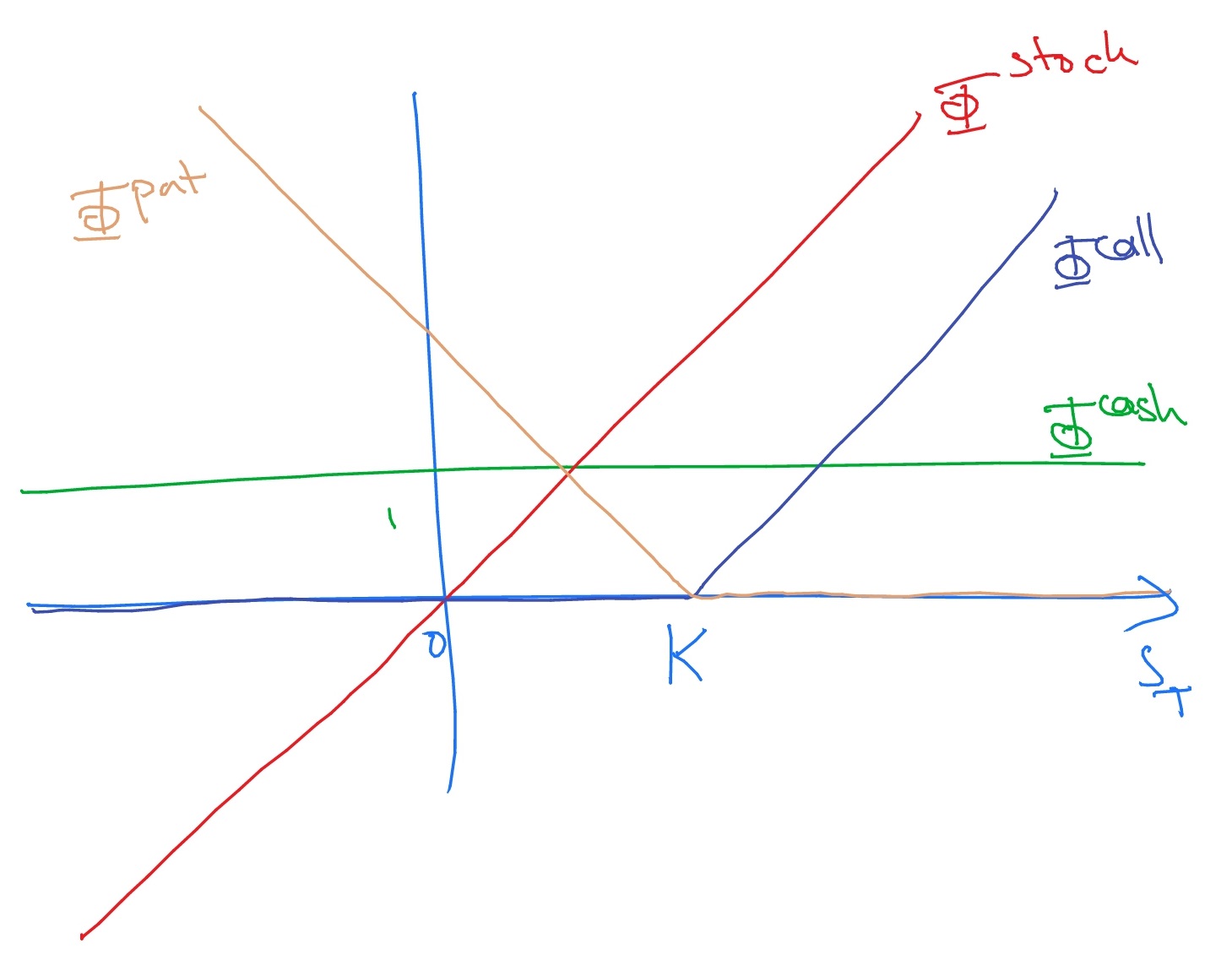
- (a) The functions $Φ^{c a s h} (S_{T}) = 1$ , $Φ^{s t o c k} (S_{T}) = S_{T}$ , $Φ^{c a l l} (S_{T}) = max (S_{T} - K, 0)$ and $Φ^{p u t} (S_{T}) = max (K - S_{T}, 0)$ look like:
- (b) In terms of functions, the put-call parity relation states that
  
  $max (K - S_{T}, 0) = max (S_{T} - K) + K - S_{T} .$
  
  To check that this holds we consider two cases.
  - • If $K \leq S_{T}$ then put-call parity states that $0 = S_{T} - K + K - S_{T}$ , which is true.
  - • If $K \geq S_{T}$ then put-call parity states that $K - S_{T} = 0 + K - S_{T}$ , which is true.
16.2 The put-call parity relation (16.1) says that

$Φ^{p u t} (S_{T}) = Φ^{c a l l} (S_{T}) + K Φ^{c a s h} (S_{T}) - Φ^{s t o c k} (S_{T}) .$

Hence,

$Π_{t}^{p u t} = Π_{t}^{c a l l} + K Π_{t}^{c a s h} - Π_{t}^{s t o c k} .$

From here, using that $Π_{t}^{c a s h} = e^{- r (T - t)}$ (corresponding to $Φ (S_{T}) = 1$ ) and $Π_{t}^{s t o c k} = S_{t}$ (corresponding to $Φ (S_{T}) = S_{T}$ ), as well as the Black-Scholes formula (15.23), we have

$\begin{aligned} Π_{t}^{p u t} & = S_{t} N [d_{1}] - K e^{- r (T - t)} N [d_{2}] + K e^{- r (T - t)} - S_{t} \\ = S_{t} (N [d_{1}] - 1) - K e^{- r (T - t)} (N [d_{2}] - 1) \\ = - S_{t} N [- d_{1}] + K e^{- r (T - t)} N [- d_{2}] . \end{aligned}$ In the last line we use that $N [x] + N [- x] = 1$ , which follows from the fact that the $N (0, 1)$ distribution is symmetric about $0$ (i.e. $P [X \leq x] + P [X \leq - x] = P [X \leq x] + P [- X \geq x] = P [X \leq x] + P [X \geq x] = 1$ ). The formula stated in the question follows from setting $t = 0$ .
16.3 Write $Φ^{c a l l, K} (S_{T}) = max (S_{T} - K, 0)$ for the contingent claim of a European call option, and $Φ^{p u t, K} (S_{T})$ for the contingent claim of a European put options, both with strike price $K$ and exercise date $T$ . Then

$Φ (S_{T}) = Φ^{c a l l, 1} (S_{T}) + Φ^{p u t, - 1} (S_{T})$

so we can hedge $Φ (S_{T})$ by holding a single call option with strike price $1$ and a single put option with strike price $- 1$ .
16.4
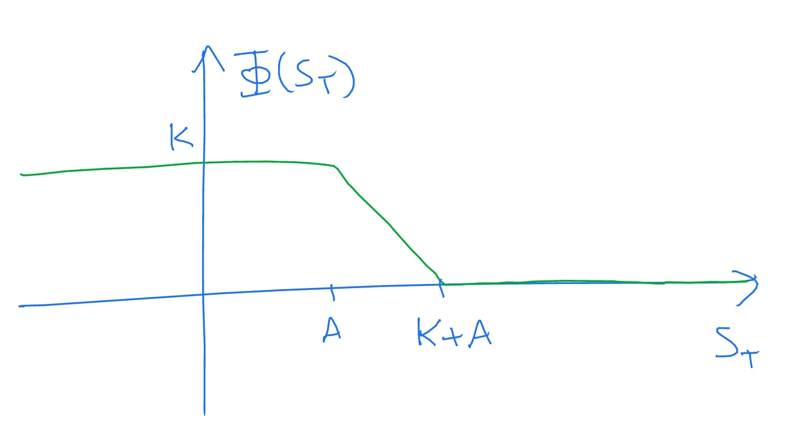
- (a) A sketch of $Φ (S_{T})$ for general $A$ looks like
  
  Let $Φ^{p u t, K} (S_{T}) = max (K - S_{T}, 0)$ denote the contingent claim corresponding to a European put option with strike price $K$ and exercise date $T$ . Then, we claim that
  
  $\begin{matrix} (C.6) & Φ (S_{T}) = Φ^{p u t, K + A} (S_{T}) - Φ^{p u t, A} (S_{T}) . \end{matrix}$
  
  The right-hand side of this equation corresponds to a portfolio of one put option with strike price $K + A$ and minus one put option with strike price $A$ . We can see that the relation (C.6) holds by using a diagram
  
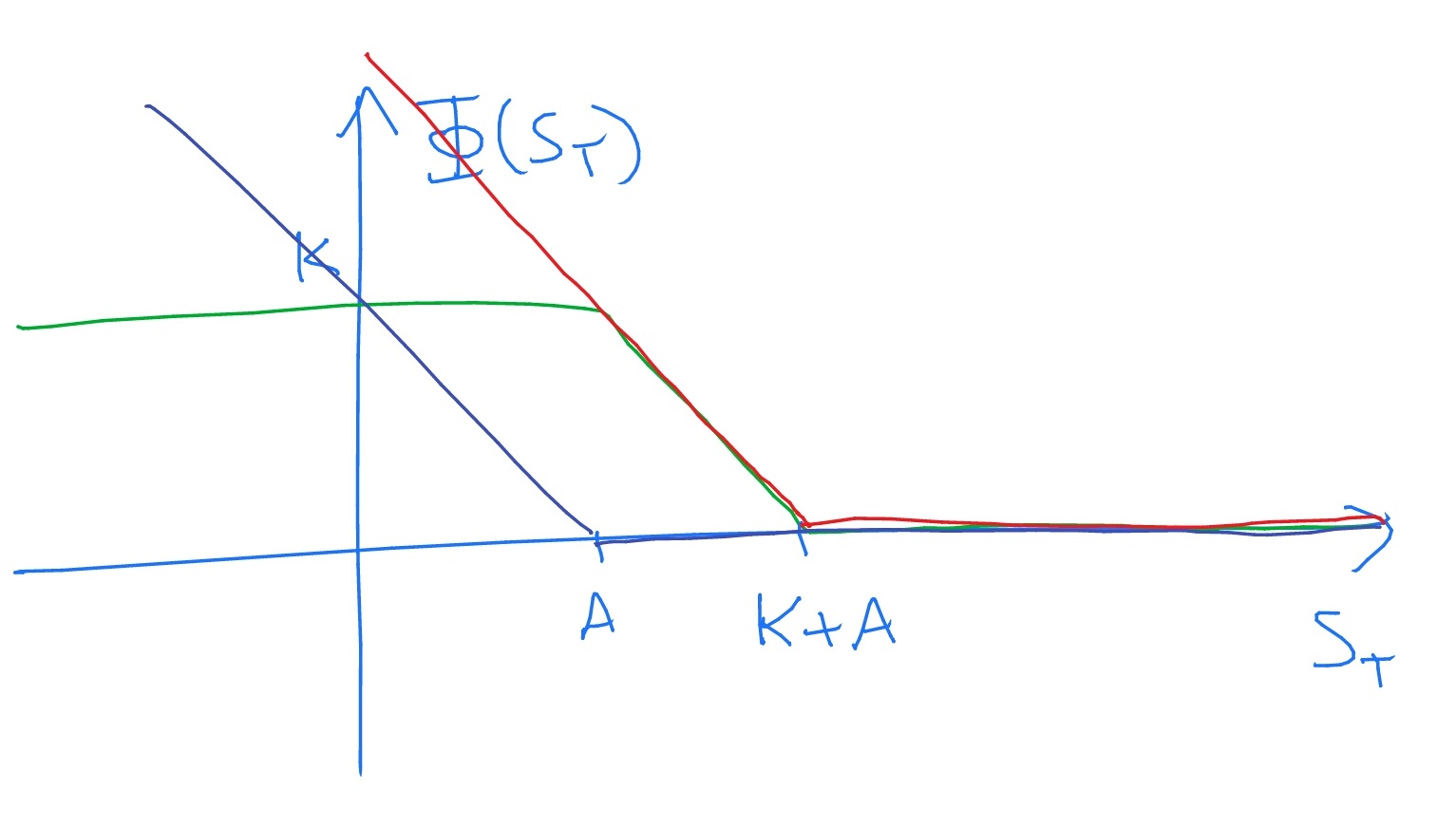
  in which the purple line $Φ^{p u t, A} (S_{T})$ is subtracted from the red line $Φ^{p u t, K + A} (S_{T})$ to obtain the green line $Φ (S_{T})$ . Alternatively, we can check it by considering three cases:
  - • If $S_{T} \leq A$ then we have $K = (K + A - S_{T}) - (A - S_{T})$ which is true.
  - • If $A \leq S_{T} \leq K + A$ then we have $K + A - S_{T} = (K + A - S_{T}) - (0)$ which is true.
  - • If $S_{T} \geq K + A$ then we have $0 = (0) - (0)$ which is true.
  Therefore, the portfolio of one put option with strike price $K + A$ and minus one put option with strike price $A$ is a replicating portfolio for $Φ (S_{T})$ .
- (b) We use put-call parity to replicate our portfolio of put options with a portfolio of cash, stock and call options. This tells us that $Φ^{p u t, K} (S_{T}) = Φ^{c a l l, K} (S_{T}) + K Φ^{c a s h} (S_{T}) + Φ^{s t o c k} (S_{T})$ . Therefore, replacing each of our put options with the equivalent amounts of cash and stock, we have
  
  $\begin{aligned} Φ^{p u t, K + A} (S_{T}) - Φ^{p u t, A} (S_{T}) & = Φ^{c a l l, K + A} (S_{T}) - Φ^{c a l l, A} (S_{T}) + (K + A - A) Φ^{c a s h} (S_{T}) - (1 - 1) Φ^{s t o c k} (S_{T}) \\ = Φ^{c a l l, K + A} (S_{T}) - Φ^{c a l l, A} (S_{T}) + K Φ^{c a s h} (S_{T}) . \end{aligned}$ Hence, $Φ (S_{T})$ can be replicated with a portfolio containing one call option with strike price $K + A$ , minus one call option with strike price $K$ , and $K$ units of cash.
- (c) Corollary 15.3.3 refers to portfolios consisting only of stocks and cash. It does not apply to portfolios that are also allowed to contain derivatives.
16.5 We can write

$Φ^{b u l l} (S_{T}) = A + max (S_{T} - A, 0) - max (S_{T} - B, 0) .$

It may help to draw a picture, in the style of 16.4. If we write $Φ^{c a l l, K} (S_{T}) = max (S_{T} - K, 0)$ and recall that $Φ^{c a s h} (S_{T}) = 1$ then we have

$Φ^{b u l l} (S_{T}) = A Φ^{c a s h} (S_{T}) + Φ^{c a l l, A} (S_{T}) - Φ^{c a l l, B} (S_{T}) .$

So, in our (constant) hedging portfolio at time $0$ we will need $A e^{- r T}$ in cash, one call option with strike price $A$ , and minus one call option with strike price $B$ .
16.9 The price computed for the contingent claim $Φ (S_{T}) = S_{t}^{β}$ in 15.3 is

$F (t, S_{t}) = S_{t}^{β} \exp (- r (T - t) (1 - β) - \frac{1}{2} σ^{2} β (T - t) (1 - β)) .$

(Recall that Theorem 15.3.1 also tells us that there is a hedging strategy $h_{t} = (x_{t}, y_{t})$ for the contingent claim with value $F (t, S_{t})$ .)

We have $F (t, s) = s^{β} \exp (- r (T - t) (1 - β) - \frac{1}{2} σ^{2} β (T - t) (1 - β))$ and we calculate

$\begin{aligned} Δ_{F} & = \frac{\partial F}{\partial s} (t, S_{t}) = β S_{t}^{β - 1} \exp (- r (T - t) (1 - β) - \frac{1}{2} σ^{2} β (T - t) (1 - β)) \\ Γ_{F} & = \frac{\partial^{2} F}{\partial s^{2}} (t, S_{t}) = β (β - 1) S_{t}^{β - 2} \exp (- r (T - t) (1 - β) - \frac{1}{2} σ^{2} β (T - t) (1 - β)) \\ Θ_{F} & = \frac{\partial F}{\partial t} (t, S_{t}) = S_{t}^{β} (1 - β) (r + \frac{1}{2} β σ^{2}) \exp (- r (T - t) (1 - β) - \frac{1}{2} σ^{2} β (T - t) (1 - β)) \\ ρ_{F} & = \frac{\partial F}{\partial r} (t, S_{t}) = - S_{t}^{β} (T - t) (1 - β) \exp (- r (T - t) (1 - β) - \frac{1}{2} σ^{2} β (T - t) (1 - β)) \\ V_{F} & = \frac{\partial F}{\partial σ} (t, S_{t}) = - S_{t}^{β} σ β (T - t) (1 - β) \exp (- r (T - t) (1 - β) - \frac{1}{2} σ^{2} β (T - t) (1 - β)) . \end{aligned}$
16.10
- (a) The underlying stock $S_{t}$ has $Δ_{S} = 1$ and $Γ_{S} = 0$ . If we add $- 2$ stock into our original portfolio with value $F$ , then its new value is $V (t, S_{t}) = F (t, S_{t}) - 2 S_{t}$ , which satisfies $Δ_{V} = Δ_{F} - 2 = 0$ .
  
  The cost of adding $- 2$ units of stock into the portfolio is $- 2 S_{t}$ .
- (b) After including an amount $w_{t}$ of stock and an amount $d_{t}$ of $D$ , we have
  
  $V (t, S_{t}) = F (t, S_{t}) + w_{t} S_{t} + d_{t} D (t, S_{t}) .$
  
  Hence, we require that
  
  $\begin{aligned} 0 & = Δ_{F} + w_{t} + d_{t} Δ_{D} = 2 + w_{t} + d_{t}, \\ 0 & = Γ_{F} + d_{t} Γ_{D} = 3 + 2 d_{t} . \end{aligned}$ The solution is $d_{t} = \frac{- 3}{2}$ and $w_{t} = \frac{- 1}{2}$ .
  
  The cost of the extra stock and units of $D$ that we have had to include is $- \frac{3}{2} D (t, S_{t}) - \frac{1}{2} S_{t}$ .
16.11
- (a) It doesn’t work because adding in an amount $z_{t}$ of $Z$ in the second step will (typically i.e. if $Δ_{Z} \neq 0$ ) destroy the delta neutrality that we gained from the first step.
- (b) Since $Z (t, S_{t}) = S_{t}$ we have
  
  $V (t, S_{t}) = F (t, S_{t}) + w_{t} W (t, S_{t}) + z_{t} S_{t},$
  
  so we require that
  
  $\begin{aligned} 0 & = \frac{\partial V}{\partial s} = Δ_{F} + w_{t} Δ_{W} + z_{t} \\ 0 & = \frac{\partial^{2} V}{\partial s^{2}} = Γ_{F} + w_{t} Γ_{W} . \end{aligned}$ The solution is easily seen to be
  
  $\begin{aligned} w_{t} & = - \frac{Γ_{F}}{Γ_{W}} \\ z_{t} & = \frac{Δ_{W} Γ_{F}}{Γ_{W}} - Δ_{F} \end{aligned}$
- (c) This idea works. As we can see from part (b), if we use stock as our financial derivative $Z (t, S_{t}) = S_{t}$ , then $Γ_{Z} = 0$ . Hence, adding in a suitable amount of stock in the second step can achieve delta neutrality without destroying the gamma neutrality obtained in the first step.
16.12 Omitted (good luck).

Chapter 19

19.1 The degrees of the nodes, in alphabetical order, are $(1, 1), (0, 2), (2, 2), (2, 0), (1, 1), (1, 2), (1, 0) .$ This gives a degree distribution

$P [D_{G} = (a, b)] = {\begin{cases} \frac{1}{7} & for (a, b) \in {(0, 2), (2, 2), (2, 0), (1, 2), (1, 0)}, \\ \frac{2}{7} & for (a, b) = (1, 1) . \end{cases}$

Sampling a uniformly random and moving along it means that the chance of ending up at a node $A$ is proportional to $\deg_{in} (A)$ . Since the graph has $8$ edges, we obtain

$\begin{aligned} P [O = n] & = {\begin{cases} \frac{1}{8} + \frac{2}{8} & for n = 0 (nodes D and G) \\ \frac{1}{8} + \frac{1}{8} & for n = 1 (nodes A and E) \\ 0 + \frac{2}{8} + \frac{1}{8} & for n = 2 (nodes B,C and F) \end{cases} \\ = {\begin{cases} \frac{3}{8} & for n = 0 \\ \frac{1}{4} & for n = 1 \\ \frac{3}{8} & for n = 2 \end{cases} \end{aligned}$
19.2 Node $Y$ can fail only if the cascade of defaults includes $X \to D \to Y$ . Given that $X$ fails, the probability that $X$ fails is $η_{3} = \frac{1}{3}$ , because $D$ has $3$ in-edges. Similarly, given that $D$ fails, the probability that $Y$ also fails is $\frac{1}{2}$ . Hence, the probability that $Y$ fails, given that $X$ fails, is $\frac{1}{6}$ .
19.3 Node $Y$ can fail if the cascade of defaults includes $X \to B \to D \to Y$ or $X \to B \to C \to D \to Y$ . Given that $X$ fails, node $B$ is certain to fail as well, since $B$ has only one in-edge. Given that $B$ fails, $C$ is certain to fail for the same reason. Therefore, the edges $(B, D)$ and $(C, D)$ are both certain to default. For each of these edges, independently, there is a chance $\frac{1}{3}$ that their own default causes $D$ to fail. The probability that $D$ fails is therefore

$\frac{1}{3} + (1 - \frac{1}{3}) \times \frac{1}{3} = \frac{5}{9} .$

Here, we condition first on if the link $B D$ causes $D$ to fail (which it does with probability $\frac{1}{3}$ ) and then, if it doesn’t (which has probability $1 - \frac{1}{3}$ ) we ask if the link $B C$ , which fails automatically and causes failure of $C D$ , causes $D$ to fail.

Given that $D$ fails, $Y$ is certain to fail. Hence, the probability that $Y$ fails, given that $X$ fails, is $\frac{5}{9}$ .
19.4 For any node of the graph (except for the root node), if its single incoming loan defaults, then its own probability of default if $α$ , independently of all else. Hence, each newly defaulted loan leads to two further defaulted loans with probability $α$ , and leads to no further defaulted loans with probability $1 - α$ . Hence, the defaulted loans form a Galton-Watson process $(Z_{n})$ with off-spring distribution $G$ , given by $P [G = 2] = α$ and $P [G = 0] = 1 - α$ , with initial state $Z_{0} = 2$ (representing the two loans which initially default when $V_{0}$ defaults).

The total number of defaulted edges is given by

$S = \sum_{n = 0}^{\infty} Z_{n} .$

Combining Lemmas 7.4.7, 7.4.6 and 7.4.8, we know that either:
- • If $E [G] > 1$ then there is positive probability that $Z_{n} \to \infty$ as $n \to \infty$ ; in this case for all large enough $n$ we have $Z_{n} \geq 1$ , and hence $S = \infty$ .
- • If $E [G] \leq 1$ then, almost surely, for all large enough $n$ we have $Z_{n} = 0$ , which means that $S < \infty$ .
We have $E [G] = 2 α$ . It is clear that the number of defaulted banks is infinite if and only if the number of defaulted loans in infinite, which has positive probability if $E [G] > 1$ . So, we conclude that there is positive probability of a catastrophic default if and only if $α > \frac{1}{2}$ .
19.5
- (a) The probability that both $B$ and $C$ fail is $\frac{1}{2} \frac{1}{2} = \frac{1}{4}$ . Given this event, the probability that both $D$ and $E$ fail is $\frac{1}{2} (1 - \frac{3}{4} \frac{3}{4} \frac{3}{4}) = \frac{37}{128}$ ; here the first term $\frac{1}{2}$ is the probability of $D$ failing (via its link to $B$ ) and the second term is one minus the probability of $E$ not failing despite all its inbound loans defaulting. Given that $D$ and $E$ both fail, the probability that $F$ fails is $1 - \frac{2}{3} \frac{2}{3} = \frac{5}{9}$ .
  
  Hence, the probability that every node fails is
  
  $\frac{1}{4} \frac{37}{128} \frac{5}{9} = \frac{185}{4608} .$
- (b) Our strategy comes in three stages: first work out the probabilities of all the possible outcomes relating to $B$ and $C$ ; secondly, do the same for $D$ and $E$ ; finally, do the same for $F$ . Each stage relies on the information obtained in the previous stage.
  
  Stage 1: The probability that $B$ fails and $C$ does not is $\frac{1}{2} \frac{1}{2} = \frac{1}{4}$ . This is also the probability that $C$ fails and $B$ does not. The probability that both $B$ and $C$ fail is also $\frac{1}{4}$ .
  
  Stage 2: Hence, the probability that $E$ fails and $D$ does not is
  
  $\frac{1}{4} (\frac{1}{4} \frac{1}{2}) + \frac{1}{4} (\frac{1}{4}) + \frac{1}{4} (\frac{1}{2}) (\frac{1}{4} + \frac{3}{4} \frac{1}{4}) = \frac{19}{128}$
  
  The three terms in the above correspond respectively to the three cases considered in the first paragraph. Similarly, the probability that $D$ fails and $E$ does not is
  
  $\frac{1}{4} (\frac{1}{2} \frac{3}{4} \frac{3}{4}) + \frac{1}{4} (0) + \frac{1}{4} (\frac{1}{2}) (\frac{3}{4} \frac{3}{4} \frac{3}{4}) = \frac{63}{512}$
  
  and the probability that both $D$ and $E$ fail is
  
  $\frac{1}{4} (\frac{1}{2}) (\frac{1}{4} + \frac{3}{4} \frac{1}{4}) + \frac{1}{4} (0) + \frac{1}{4} (\frac{1}{2}) (1 - \frac{3}{4} \frac{3}{4} \frac{3}{4}) = \frac{65}{512}$
  
  .
  
  Stage 3: Finally, considering these three cases in turn, the probability that $F$ fails is
  
  $\frac{19}{128} (\frac{1}{3}) + \frac{63}{512} (\frac{1}{3}) + \frac{65}{512} (1 - \frac{2}{3} \frac{2}{3}) = \frac{371}{2304} .$

Stochastic Processes and Financial Mathematics (part two)

Chapter C Solutions to exercises (part two)

Chapter 11

Chapter 12

Chapter 13

Chapter 14

Chapter 15

Chapter 16

Chapter 19

Stochastic Processes and Financial Mathematics
(part two)