Stochastic Processes and Financial Mathematics
(part one)

7.4 Long term behaviour of stochastic processes

Our next step is to use the martingale convergence theorem to look at the behaviour as \(t\to \infty \) of various stochastic processes. We will begin with Roulette, from Section 7.2, and then move on to the trio of stochastic processes (random walks, urns, branching processes) that we introduced in Chapter 4.

One fact, from real analysis, that we will find useful is the following:

Proof: Put \(\epsilon =\frac 13\) into the definition of a convergent real sequence, and we obtain that there exists \(N\in \N \) such that \(|a_n-a|\leq \frac 13\) for all \(n\geq N\). Hence, for \(n\geq N\) we have

\begin{align*} |a_n-a_{n+1}|=|a_n-a+a-a_{n+1}| &\leq |a_n-a|+|a-a_{n+1}|\\ &\leq \tfrac 13+\tfrac 13\\ &=\tfrac 23. \end{align*} Since \(\frac 23<1\), and \(a_n\) takes only integer values, this means that \(a_n=a_{n+1}\). Since this holds for all \(n\geq N\), we must have \(a_N=a_{N+1}=a_{N+2}=\ldots \), which means that \(a_n\to a_N\) as \(N\to \infty \) (and hence \(a=a_N\)).   ∎

Long term behaviour of Roulette

Let us think about what happens to our Roulette player, from Section 7.2.

Recall that our gambler bets an amount \(C_{n-1}\in \mc {F}_{n-1}\) on play \(n\). On each play, our gambler increases his wealth, by \(C_{n-1}\), with probability \(\frac {18}{37}\), or decreases his wealth, by \(C_{n-1}\), with probability \(\frac {19}{37}\). We showed in Section 7.2 that his profit/loss after \(n\) plays was a supermartingale, \((C\circ M)_n.\) Thus, if our gambler starts with an amount of money \(K\in \N \) at time \(0\), then at time \(n\) they have an amount of money given by

\begin{equation} \label {eq:roulette_winnings} W_n=K+(C\circ M)_n. \end{equation}

We’ll assume that our gambler keeps betting until they run out of money, so we have \(C_n\geq 1\) and \(W_n\geq 0\) for all \(n\) before they run out of money (and, if and when they do run out, \(C_n=0\) for all remaining \(n\)). Since money is a discrete quantity, we can assume that \(K\) and \(C_n\) are integers, hence \(W_n\) is also always an integer.

From Section 7.2 we know that \((C\circ M)_n\) is a supermartingale, hence \(W_n\) is also a supermartingale. Since \(W_n\geq 0\) we have \(\E [|W_n|]=\E [W_n]\leq \E [W_0]\) so \((W_n)\) is uniformly bounded in \(L^1\). Hence, by the martingale convergence theorem, \(W_n\) is almost surely convergent.

By Lemma 7.4.1, the only way that \(W_n\) can converge is if it becomes constant, eventually. Since each play results in a win (an increase) or a loss (a decrease) the only way \(W_n\) can become eventually constant is if our gambler has lost all his money i.e. for some (random) \(N\in \N \), for all \(n\geq N\), we have \(W_n=0\). Thus:

Long term behaviour of urn processes

We will look at the Pólya urn process introduced in Section 4.2. Recall that we start our urn with \(2\) balls, one red and one black. Then, at each time \(n=1,2,\ldots ,\) we draw a ball, uniformly at random, from the urn, and replace it alongside an additional ball of the same colour. Thus, at time \(n\) (which means: after the \(n^{th}\) draw is completed) the urn contains \(n+2\) balls.

Recall also that we write \(B_n\) for the number of red balls in the urn at time \(n\), and

\begin{equation} \label {eq:urn_Mn2} M_n=\frac {B_n}{n+2} \end{equation}

for the fraction of red balls in the urn at time \(n\). We have shown in Section 4.2 that \(M_n\) is a martingale. Since \(M_n\in [0,1]\), we have \(\E [|M_n|]\leq 1\), hence \((M_n)\) is uniformly bounded in \(L^1\) and the martingale convergence theorem applies. Therefore, there exists a random variable \(M_\infty \) such that \(M_n\stackrel {a.s.}{\to }M_\infty \). We will show that:

We now aim to prove Proposition 7.4.3, which means we must find out the distribution of \(M_\infty \). In order to do so, we will use Lemma 6.1.2, which tells us that \(M_n\stackrel {d}{\to }M_\infty \), that is

\begin{align} \label {eq:urn_Mconvd} \P [M_n\leq x]\to \P [M_\infty \leq x] \end{align} for all \(x\), except possibly those for which \(\P [M_\infty =x]>0\). We will begin with a surprising lemma that tells us the distribution of \(B_n\). Then, using (7.6), we will be able to find the distribution of \(M_n\), from which (7.7) will then tell us the distribution of \(M_\infty \).

Proof: Let \(A\) be the event that the first \(k\) balls drawn are red, and the next \(j\) balls drawn are black. Then,

\begin{equation} \label {eq:urn_rb_draws} \P [A]=\frac {1}{2}\frac {2}{3}\ldots \frac {k}{k+1}\frac {1}{k+2}\frac {2}{k+3}\ldots \frac {j}{j+k+1}. \end{equation}

Here, each fraction corresponds (in order) to the probability of getting a red/black ball (as appropriate) on the corresponding draw, given the results of previous draws. For example, \(\frac 12\) is the probability that the first draw results in a red ball, after which the urn contains \(2\) red balls and \(1\) black ball, so \(\frac 23\) is the probability that the second draw results in a red ball, and so on. From (7.8) we have \(\P [A]=\frac {j!k!}{(j+k+1)!}\).

Here is the clever part: we note that drawing \(k\) red balls and \(j\) black balls, in the first \(j+k\) draws but in a different order, would have the same probability. We would simply obtain the numerators in (7.8) in a different order. There are \(\binom {j+k}{k}\) possible different orders (i.e. we must choose \(k\) time-points from \(j+k\) times at which to pick the red balls). Hence, the probability that we draw \(k\) red and \(j\) black in the first \(j+k\) draws is

\[\binom {j+k}{k}\frac {j!k!}{(j+k+1)!}=\frac {(j+k)!}{k!(j+k-k)!}\frac {j!k!}{(j+k+1)!}=\frac {1}{j+k+1}.\]

We set \(j=n-k\), to obtain the probability of drawing (and thus adding) \(k\) red balls within the first \(j+k=n\) draws. Hence \(\P [B_n=k+1]=\frac {1}{n+1}\) for all \(k=0,1,\ldots ,n\). Setting \(k'=k+1\), we recover the statement of the lemma.   ∎

Proof:[Of Proposition 7.4.3.] Now that we know the distribution of \(B_n\), we can use (7.6) to find out the distribution of \(M_n\). Lemma 7.4.5 tells us that \(B_n\) is uniformly distribution on the set \(\{1,\ldots ,n+1\}\). Hence \(M_n\) is uniform on \(\{\frac {1}{n+2},\frac {2}{n+2},\ldots ,\frac {n+1}{n+2}\}\). This gives us that, for \(x\in (0,1)\),

\begin{align*} \P [M_n\leq x]=\frac {1}{n+1} \times \lfloor x(n+2) \rfloor . \end{align*} Here, \(\lfloor x(n+2) \rfloor \), which denotes the integer part of \(x(n+2)\), is equal to the number of elements of \(\{\frac {1}{n+2},\frac {2}{n+2},\ldots ,\frac {n+1}{n+2}\}\) that are \(\leq x\). Since \(x(n+2)-1\leq \lfloor x(n+2)\rfloor \leq x(n+2)\) we obtain that

\[\frac {x(n+2)-1}{n+1}\leq \P [M_n\leq x]\leq \frac {x(n+2)}{n+1}\]

and the sandwich rule tells us that \(\lim _{n\to \infty }\P [M_n\leq x]=x\). By (7.7), this means that

\[\P [M_\infty \leq x]=x\quad \text { for all }x\in (0,1).\]

Therefore, \(M_\infty \) has a uniform distribution on \((0,1)\). This proves Proposition 7.4.3.   ∎

Extensions and applications of urn processes

We could change the rules of our urn process, to create a new kind of urn – for example whenever we draw a red ball we could add two new red balls, rather than just one. Urn processes are typically very ‘sensitive’, meaning that a small change in the process, or its initial conditions, can have a big effect on the long term behaviour. You can investigate some examples of this in exercises 7.7, 7.8 and 7.9.

Urn processes are often used in models in which the ‘next step’ of the process depends on sampling from its current state. Recall that in random walks we have \(S_{n+1}=S_n+X_{n+1}\), where \(X_{n+1}\) is independent of \(S_n\); so for random walks the next step of the process is independent of its current state. By contrast, in Pólya’s urn, whether the next ball we add is red (or black) depends on the current state of the urn; it depends on which colour ball we draw.

For example, we might look at people choosing which restaurant they have dinner at. Consider two restaurants, say Café Rouge (which is red) and Le Chat Noir (which is black). We think of customers in Café Rouge as red balls, and customers in Le Chat Noir as black balls. A newly arriving customer (i.e. a new ball that we add to the urn) choosing which restaurant to visit is more likely, but not certain, to choose the restaurant which currently has the most customers.

Other examples include the growth of social networks (people tend to befriend people who already have many friends), machine learning (used in techniques for becoming successively more confident about partially learned information), and maximal safe dosage estimation in clinical trials (complicated reasons). Exercise 7.8 features an example of an urn process that is the basis for modern models of evolution (successful organisms tend to have more descendants, who are themselves more likely to inherit genes that will make them successful).

Long term behaviour of Galton-Watson processes

The martingale convergence theorem can tell us about the long term behaviour of stochastic processes. In this section we focus on the Galton-Watson process, which we introduced in Section 4.3.

Let us recall the notation from Section 4.3. Let \(X^n_i\), where \(n,i\ge 1\), be i.i.d. nonnegative integer-valued random variables with common distribution \(G\). Define a sequence \((Z_n)\) by \(Z_0=1\) and

\begin{equation} \label {eq:gw_iterative_defn} Z_{n+1} = \left \{ \begin{array}{ll} X^{n+1}_1 + \ldots + X^{n+1}_{Z_n}, & \mbox { if $Z_n>0$} \\ 0, & \mbox { if $Z_n=0$} \end {array} \right . \end{equation}

Then \((Z_n)\) is the Galton-Watson process. In Section 4.3 we showed that, writing \(\mu =\E [G]\),

\[M_n=\frac {Z_n}{\mu ^n}\]

was a martingale with mean \(\E [M_n]=1\).

We now look to describe the long term behaviour of the process \(Z_n\), meaning that we want to know how \(Z_n\) behaves as \(n\to \infty \). We’ll consider three cases: \(\mu <1\), \(\mu =1\), and \(\mu >1\). Before we start, its important to note that, if \(Z_N=0\) for any \(N\in \N \), then \(Z_n=0\) for all \(n\geq N\). When this happens, it is said that the process dies out.

We’ll need the martingale convergence theorem. We have that \(M_n\) is a martingale, with expected value \(1\), and since \(M_n\geq 0\) we have \(\E [|M_n|]=1\). Hence, \((M_n)\) is uniformly bounded in \(L^1\) and by the martingale convergence theorem (Theorem 7.3.4) we have that the almost sure limit

\[\lim \limits _{n\to \infty }M_n=M_\infty \]

exists. Since \(M_n\geq 0\), we have \(M_\infty \in [0,\infty )\).

For the rest of this section, we’ll assume that the offspring distribution \(G\) is not deterministic. Obviously, if \(G\) was deterministic and equal to say, \(c\), then we would simply have \(Z_n=c^n\) for all \(n\).

Proof: In this case \(M_n=Z_n\). So, we have \(Z_n\to M_\infty \) almost surely. The offspring distribution is not deterministic, so for as long as \(Z_n\neq 0\) the value of \(Z_n\) will continue to change over time. Each such change in value is of magnitude at least \(1\), hence by Lemma 7.4.1 the only way \(Z_n\) can converge is if \(Z_n\) is eventually zero. Therefore, since \(Z_n\) does converge, in this case we must have \(\P [Z_n\text { dies out}]=1\) (and \(M_\infty =0\)).   ∎

Sketch of Proof: Recall our graphical representation of the Galton-Watson process in Section 4.3. Here’s the key idea: when \(\mu <1\), on average we expect each individual to have less children than when \(\mu =1\). Therefore, if the Galton-Watson process dies out when \(\mu =1\) (as is the case, from Lemma 7.4.6), it should also die out when \(\mu <1\).

Our idea is not quite a proof, because the size of the Galton-Watson process \(Z_n\) is random, and not necessarily equal to its expected size \(\E [Z_n]=\mu ^n\). To make the idea into a proof we will need to find two Galton-Watson processes, \(Z_n\) and \(\wt {Z}_n\), such that \(0\leq Z_n\leq \wt {Z}_n\), with \(\mu <1\) in \(Z_n\) and \(\mu =1\) in \(\wt {Z}_n\). Then, when \(\wt {Z}_n\) becomes extinct, so does \(Z_n\). This type of argument is known as a coupling, meaning that we use one stochastic process to control another. See exercise 7.15 for how to do it.   ∎

Proof: The first step of the argument is to show that, for all \(n\in \N \),

\begin{equation} \label {eq:gw_2nd_iterate} \E [M_{n+1}^2]=\E [M_n^2]+\frac {\sigma ^2}{\mu ^{n+2}}. \end{equation}

You can find this calculation as exercise 7.13. It is similar to the calculation that we did to find \(\E [M_n]\) in Section 4.3, but a bit harder because of the square.

By iterating (7.10) and noting that \(\E [M_0]=1\), we obtain that

\[\E [M_{n+1}^2]=1+\sum _{i=1}^n\frac {\sigma ^2}{\mu ^{i+2}}.\]

Hence,

\[\E [M_{n+1}^2]\leq 1+\frac {\sigma ^2}{\mu ^2}\sum _{i=1}^\infty \frac {1}{\mu ^i},\]

which is finite because \(\mu >1\). Therefore, \((M_n)\) is uniformly bounded in \(L^2\), and the second martingale convergence theorem applies. In particular, this gives us that

\[\E [M_n]\to \E [M_\infty ].\]

Noting that \(\E [M_n]=1\) for all \(n\), we obtain that \(\E [M_\infty ]=1\). Hence, \(\P [M_\infty >0]>0\). On the event that \(M_\infty >0\), we have \(M_n=\frac {Z_n}{\mu ^n}\to M_\infty >0\). Since \(\mu ^n\to \infty \), this means that when \(M_\infty >0\) we must also have \(Z_n\to \infty \). Hence, \(\P [Z_n\to \infty ]>0\).   ∎

The behaviour \(Z_n\to \infty \) is often called ‘explosion’, reflecting the fact that (when it happens) each generation tends to contain more and more individuals than the previous one. The case of \(\mu >1\) and \(\sigma ^2=\infty \) behaves in the same way as Lemma 7.4.8, but the proof is more difficult and we don’t study it in this course.

Extensions and applications of the Galton-Watson process

The Galton-Watson process can be extended in many ways. For example, we might vary the offspring distribution used in each generation, or add a mechanism that allows individuals to produce their children gradually across multiple time steps. The general term for such processes is ‘branching processes’. Most branching processes display the same type of long-term behaviour as we have uncovered in this section: if the offspring production is too low (on average) then they are sure to die out, but, if the offspring production is high enough that dying out is not a certainty then (instead) there is a chance of explosion to \(\infty \).

Branching processes are the basis of stochastic models in which existing objects reproduce, or break up, into several new objects. Examples are the spread of contagious disease, crushing rocks, nuclear fission, tumour growth, and so on. In Chapter 19 (which is part of MAS61023 only) we will use branching processes to model contagion of unpaid debts in banking networks.

Branching processes are used by biologists to model population growth, and they are good models for populations that are rapidly increasing in size. (For populations that have reached a roughly constant size, models based on urn processes, such as that of exercise 7.8, are more effective.)

Long term behaviour of random walks \(\offsyl \)

We now consider the long term behaviour of random walks. This section won’t include proofs, and for that reason it is marked with a \(\offsyl \) and is off syllabus. We will cover this chapter in lectures, because it contain interesting information that provides intuition for (on-syllabus) results in future chapters. For those of you taking MAS61023 a full set of proofs, using some new techniques, are included in your independent reading in Chapters 8 and 9. However, some parts of the results discussed below can be proved using the techniques we’ve already studied; exercises of this type are on-syllabus for everyone, and you’ll see some at the end of this chapter.

Firstly, take \(S_n\) to be the simple symmetric random walk. It turns out that \(S_n\) will oscillate as \(n\to \infty \), and that the magnitude of the largest oscillations will tend to infinity as \(n\to \infty \) (almost surely). So, our picture of the long-term behaviour of the symmetric random walk looks like:

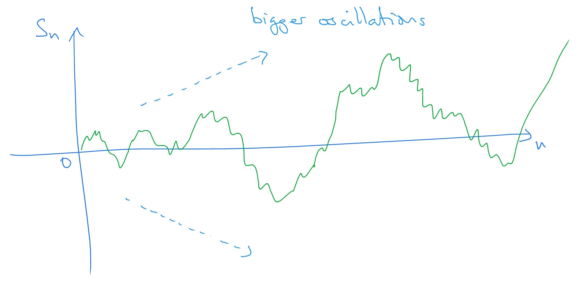
Note that we draw the picture as a continuous line, for convenience, but in fact the random walk is jumping between integer values.

Next, let \(S_n\) be the asymmetric random walk, with \(p>q\), so the walk drifts upwards. The asymmetric random walk also experiences oscillations growing larger and larger, but the drift upwards is strong enough that, in fact \(S_n\stackrel {a.s.}{\to }\infty \) as \(n\to \infty \). So, our picture of the long-term behaviour of the asymmetric random walk looks like:

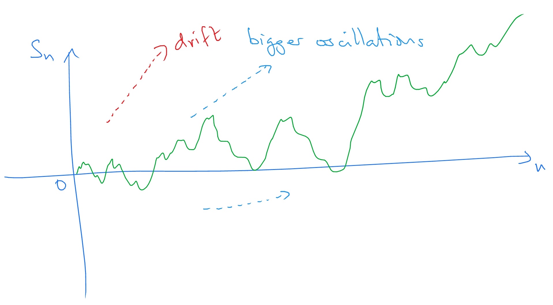
Of course, if \(q<p\) then \(S_n\) would drift downwards, and then \(S_n\stackrel {a.s.}{\to }-\infty \).

Extensions and applications of random walks

Random walks can be extended in many ways, such as by adding an environment that influences the behaviour of the walk (e.g. reflection upwards from the origin as in exercise 4.5, slower movements when above \(0\), etc), or by having random walkers that walk around a graph (\(\Z \), in our case above). More complex extensions involve random walks that are influenced by their own history, for example by having a preference to move into sites that they have not yet visited. In addition, many physical systems can be modelled by systems of several random walks, that interact with each other, for example a setup with multiple random walks happening at the same time (but started from different points in space) in which, whenever random walkers meet, both of them suddenly vanish.

Random walks are the basis of essentially all stochastic modelling that involves particles moving around randomly in space. For example, atoms in gases and liquids, animal movement, heat diffusion, conduction of electricity, transportation networks, internet traffic, and so on.

In Chapters 15 and 16 we will use stock price models that are based on ‘Brownian motion’, which is itself introduced in Chapter 11 and is the continuous analogue of the symmetric random walk (i.e. no discontinuities). We’ll come back to the idea of atoms in gases and liquids in Section 11.1, and we’ll also briefly look at heat diffusion in Section 11.3.