Stochastic Processes and Financial Mathematics
(part one)

7.3 The martingale convergence theorem

In this section, we are concerned with almost sure convergence of supermartingales \((M_n)\) as \(n\to \infty \). Naturally, martingales are a special case and submartingales can be handled through multiplying by \(-1\). We’ll need the following definition:

As usual, we’ll mostly only be concerned with the cases \(p=1,2\).

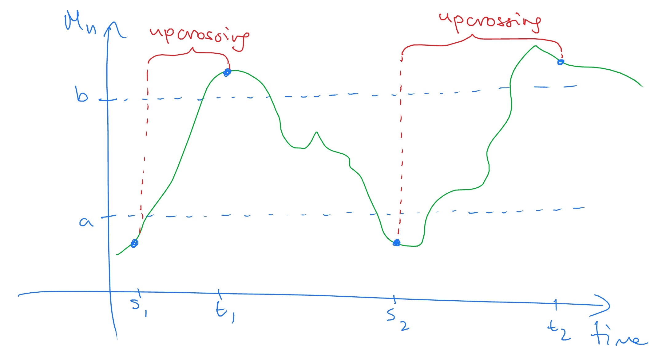
Let \((M_n)\) be a stochastic process and fix \(a<b\). We define \(U_N[a,b]\) to be the number of upcrossings made in the interval \([a,b]\) by \(M_1,\dots ,M_N\). That is, \(U_n[a,b]\) is the largest \(k\) such there exists

\[ 0\leq s_1 < t_2 < \ldots < s_k < t_k \leq N \hspace {1pc}\text { such that }\hspace {1pc} M_{s_i}\leq a, M_{t_i}> b\;\text { for all }i=1,\ldots ,k. \]

This definition is best understood through a picture:

Note that, for convenience, we draw \(M_n\) as a continuous (green line) although in fact it only changing value at discrete times.

Studying upcrossings is key to establishing almost sure convergence of supermartingales. To see why upcrossings are important, note that if \((c_n)\sw \R \) is a (deterministic) sequence and \(c_n\to c\), for some \(c\in \R \), then there is no interval \([a,b]\) \(a<b\) such that \((c_n)_{n=1}^\infty \) makes infinitely many upcrossings of \([a,b]\); if there was then \((c_n)\) would oscillate and couldn’t converge.

Note that \(U_N[a,b]\) is an increasing function of \(N\), and define \(U_\infty [a,b]\) by

\begin{equation} \label {eq:UNU} U_\infty [a,b](\omega )=\lim _{N\uparrow \infty } U_N[a,b](\omega ). \end{equation}

This is an almost surely limit, since it holds for each \(\omega \in \Omega \). With this definition, \(U_\infty [a,b]\) could potentially be infinite, but we can prove that it is not.

Proof: Let \(C_1=\1\{M_0<a\}\) and recursively define

\[ C_n=\1\{C_{n-1}=1,M_{n}\leq b\}+\1\{C_{n-1}=0,M_{n}\leq a\}. \]

The behaviour of \(C_n\) is that, when \(X\) enters the region below \(a\), \(C_n\) starts taking the value \(1\). It will continue to take the value \(1\) until \(M\) enters the region above \(b\), at which point \(C_n\) will start taking the value \(0\). It will continue to take the value \(0\) until \(M\) enters the region below \(a\), and so on. Hence,

\begin{equation} \label {eq:Doobup_eq} (C\circ M)_N=\sum _{k=1}^N C_{k-1}(M_{k}-M_{k-1}) \ge (b-a)U_N[a,b]-|M_N-a|. \end{equation}

That is, each upcrossing of \([a,b]\) by \(M\) picks up at least \((b-a)\); the final term corresponds to an upcrossing that \(M\) might have started but not finished.

Note that \(C_n\) is adapted, bounded and non-negative. Hence, by Theorem 7.1.1 we have that \(C\circ M\) is a supermartingale. Thus \(\E [(C\circ M)_N]\le 0\), which combined with (7.2) proves the given result.   ∎

Proof: From Lemma 7.3.2 we have

\begin{equation} \label {eq:UNbound} (b-a) \E [U_N[a,b]]\leq |a|+\sup _{n\in \N }\E |M_n|. \end{equation}

We have that \(U_N[a,b]\) is increasing, as \(N\) increases, and the definition of \(U_\infty [a,b]\) in (7.1) gives that that \(U_N[a,n]\to U_\infty [a,b]\) almost surely as \(N\to \infty \). Hence, by the monotone convergence theorem, \(\E [U_N[a,b]]\to \E [U_\infty [a,b]]\), and so by letting \(N\to \infty \) in (7.3) we have

\[(b-a)\E [U_\infty [a,b]]\leq |a|+\sup _{n\in \N }\E |M_n|<\infty ,\]

which implies that \(\P [U_\infty [a,b]<\infty ]=1\).   ∎

Essentially, Lemma 7.3.3 says that the paths of \(M\) cannot oscillate indefinitely. This is the crucial ingredient of the martingale convergence theorem.

Proof: Define

\[\Lambda _{a,b}=\{\om :\text { for infinitely many }n, M_n(\omega )<a\}\cap \{\om :\text { for infinitely many }n, M_n(\omega )>b\}.\]

We observe that \(\Lambda _{a,b}\sw \{U_\infty [a,b]=\infty \}\), which has probability 0 by Lemma 7.3.3. But since

\[ \{\om : M_n(\om ) \mbox { does not converge to a limit in } [-\infty ,\infty ]\} = \bigcup _{\stackrel {a,b\in \mathbb {Q}}{a<b}} \Lambda _{a,b}, \]

we have that

\[ \P [M_n \mbox { converges to some } M_\infty \in [-\infty ,+\infty ]]=1\]

which proves the first part of the theorem.

To prove the second part we will use an inequality that holds for any convergent sequence \(M_n\stackrel {a.s.}{\to } M_\infty \) of random variables:

\begin{equation} \label {eq:fatou_subst} \E [|M_\infty |]\leq \sup _{n\in \N }\E [|M_n|]. \end{equation}

This inequality can be proved using the monotone convergence theorem and some careful analysis, see exercise 7.14. Since we assumed that \((M_n)\) is uniformly bounded in \(L^1\), (7.4) gives us that \(\E [|M_\infty |]<\infty \). Hence, \(\P [|M_\infty |=\infty ]=0\) (or else the expected value would be infinite).   ∎

One useful note is that if \(M_n\) is a non-negative supermartingale then we have \(\E [|M_n|]=\E [M_n]\le \E [M_0]\), so in this case \(M\) is uniformly bounded in \(L^1\).

Theorem 7.3.4 has one big disadvantage: it cannot tell us anything about the limit \(M_\infty \), except that it is finite. To gain more information about \(M_\infty \), we need an extra condition.

The proof of Corollary 7.3.5 is outside of the scope of our course.