Stochastic Processes and Financial Mathematics
(part one)
7.2 Roulette
The martingale transform is a useful theoretical tool (see e.g. Sections 7.3, 8.2 and 12.1), but it also provides a framework to model casino games. We illustrate this with Roulette.
In roulette, a metal ball lies inside of a spinning wheel. The wheel is divided into 37 segments, of which 18 are black, 18 are red, and 1 is green. The wheel is spun, and the ball spins with it, eventually coming to rest in one of the 37 segments. If the roulette wheel is manufactured properly, the ball lands in each segment with probability \(\frac {1}{37}\) and the result of each spin is independent.
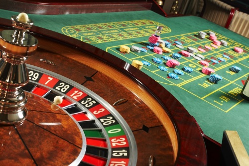
On each spin, a player can bet an amount of money \(C\). The player chooses either red or black. If the ball lands on the colour of their choice, they get their bet of \(C\) returned and win an additional \(C\). Otherwise, the casino takes the money and the player gets nothing.
The key point is that players can only bet on red or black. If the ball lands on green, the casino takes everyones money.
In each round of roulette, a players probability of winning is \(\frac {18}{37}\) (it does not matter which colour they pick). Let \((X_n)\) be a sequence of i.i.d. random variables such that
\[ X_n= \begin {cases} 1 & \text { with probability }\frac {18}{37}\\ -1 & \text { with probability }\frac {19}{37}\\ \end {cases} \]
Naturally, the first case corresponds to the player winning game \(n\) and the second to losing. We define
\[M_n=\sum \limits _{i=1}^n X_n.\]
Then, the value of \(M_n-M_{n-1}=X_n\) is \(1\) if the player wins game \(n\) and \(-1\) if they lose. We take our filtration to be generated by \((M_n)\), so \(\mc {F}_n=\sigma (M_i\-i\leq n)\).
A player cannot see into the future. So the bet they place on game \(n\) must be chosen before the game is played, at time \(n-1\) – we write this bet as \(C_{n-1}\), and require that it is \(\mc {F}_{n-1}\) measurable. Hence, \(C\) is adapted. The total profit/loss of the player over time is the martingale transform
\[(C\circ M)_n=\sum \limits _{i=1}^n C_{i-1}(M_i-M_{i-1}).\]
We’ll now show that \((M_n)\) is a supermartingale. We have \(M_n\in m\mc {F}_n\) and since \(|M_n|\leq n\) we also have \(M_n\in L^1\). Lastly,
\(\seteqnumber{0}{7.}{0}\)\begin{align*} \E [M_{n+1}|\mc {F}_n] &=\E \l [X_{n+1}+M_n\|\mc {F}_n\r ]\\ &=\E [X_{n+1}|\mc {F}_n]+M_n\\ &=\E [X_{n+1}]+M_n\\ &\leq M_n. \end{align*} Here, the second line follows by linearity and the taking out what is known rule. The third line follows because \(X_{n+1}\) is independent of \(\mc {F}_n\), and the last line follows because \(\E [X_{n+1}]=\frac {-1}{37}<0\).
So, \((M_n)\) is a supermartingale and \((C_n)\) is adapted. Theorem 7.1.1 applies and tells us that \((C\circ M)_n\) is a supermartingale. We’ll continue this story in Section 7.4.
-
Remark 7.2.2 There have been ingenious attempts to win money at Roulette, often through hidden technology or by exploiting mechanical flaws (which can slightly bias the odds), mixed with probability theory.
In 1961, Edward O. Thorp (a professor of mathematics) and Claude Shannon (a professor of electrical engineering) created the worlds first wearable computer, which timed the movements of the ball and wheel, and used this information to try and predict roughly where the ball would land. Here’s the machine itself:
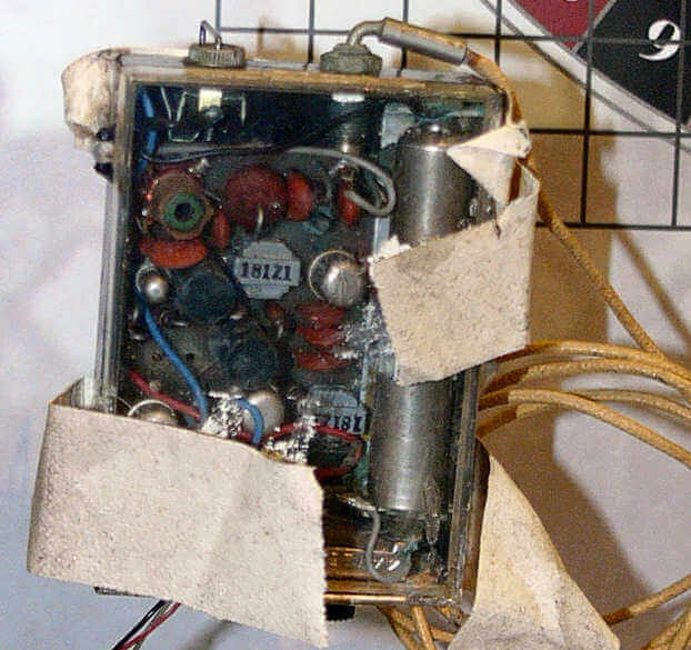
Information was input to the computer by its wearer, who silently tapped their foot as the Roulette wheel spun. By combining this information with elements of probability theory, they believed they could consistently ‘beat the casino’. They were very successful, and obtained a return of \(144\%\) on their bets. Their method is now illegal; at the time it was not, because no-one had even thought it might be possible.
Of course, most gamblers are not so fortunate.