Stochastic Processes and Financial Mathematics
(part one)
1.2 The one-period market
Let’s replace our betting game by a more realistic situation. This will require us to define some terminology. Our convention, for the whole of the course, is that when we introduce a new piece of financial terminology we’ll write it in bold.
A market is any setting where it is possible to buy and sell one or more quantities. An object that can be bought and sold is called a commodity. For our purposes, we will always define exactly what can be bought and sold, and how the value of each commodity changes with time. We use the variable \(t\) for time.
It is important to realize that money itself is a commodity. It can be bought and sold, in the sense that it is common to exchange money for some other commodity. For example, we might exchange some money for a new pair of shoes; at that same instant someone else is exchanging a pair of shoes for money. When we think of money as a commodity we will usually refer to it as cash or as a cash bond.
In this section we define a market, which we’ll then study for the rest of Chapter 1. It will be a simple market, with only two commodities. Naturally, we have plans to study more sophisticated examples, but we should start small!
Unlike our coin toss, in our market we will have time. As time passes money earns interest, or if it is money that we owe we will be required to pay interest. We’ll have just one step of time in our simple market. That is, we’ll have time \(t=0\) and time \(t=1\). For this reason, we will call our market the one-period market.
Let \(r>0\) be a deterministic constant, known as the interest rate. If we put an amount \(x\) of cash into the bank at time \(t=0\) and leave it there until time \(t=1\), the bank will then contain
\[x(1+r)\]
in cash. The same formula applies if \(x\) is negative. This corresponds to borrowing \(C_0\) from the bank (i.e. taking out a loan) and the bank then requires us to pay interest on the loan.
Our market contains cash, as its first commodity. As its second, we will have a stock. Let us take a brief detour and explain what is meant by stock.
Firstly, we should realize that companies can be (and frequently are) owned by more than one person at any given time. Secondly, the ‘right of ownership of a company’ can be broken down into several different rights, such as:
-
• The right to a share of the profits.
-
• The right to vote on decisions concerning the companies future – for example, on a possible merger with another company.
A share is a proportion of the rights of ownership of a company; for example a company might split its rights of ownership into 100 equal shares, which can then be bought and sold individually. The value of a share will vary over time, often according to how the successful the company is. A collection of one or more shares in a company is known as stock.
We allow the amount of stock that we own to be any real number. This means we can own a fractional amount of stock, or even a negative amount of stock. This is realistic: in the same way as we could borrow cash from a bank, we can borrow stock from a stockbroker! We don’t pay any interest on borrowed stock, we just have to eventually return it. (In reality the stockbroker would charge us a fee but we’ll pretend they don’t, for simplicity.)
The value or worth of a stock (or, indeed any commodity) is the amount of cash required to buy a single unit of stock. This changes, randomly:
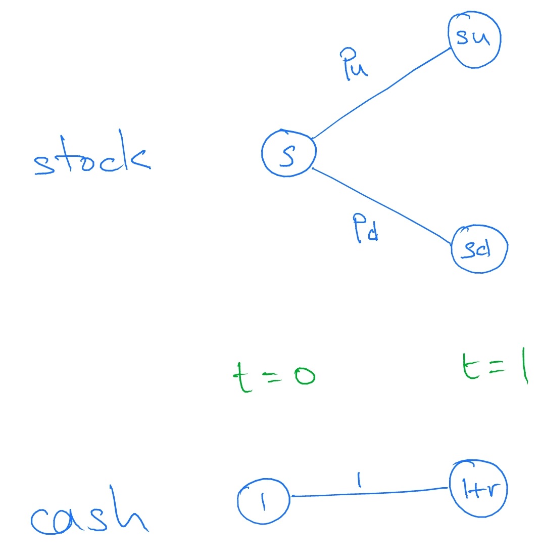
Let \(u>d>0\) and \(s>0\) be deterministic constants. At time \(t=0\), it costs \(S_0=s\) cash to buy one unit of stock. At time \(t=1\), one unit of stock becomes worth
\[S_1= \begin {cases} su & \text {with probability }p_u,\\ sd & \text {with probability }p_d.\\ \end {cases} \]
of cash. Here, \(p_u,p_d>0\) and \(p_u+p_d=1\).
We can represent the changes in value of cash and stocks as a tree, where each edge is labelled by the probability of occurrence.
To sum up, in the one-period market it is possible to trade stocks and cash. There are two points in time, \(t=0\) and \(t=1\).
-
• If we have \(x\) units of cash at time \(t=0\), they will become worth \(x(1+r)\) at time \(t=1\).
-
• If we have \(y\) units of stock, that are worth \(yS_0=sy\) at time \(t=0\), they will become worth
\[yS_1= \begin {cases} ysu & \text {with probability }p_u,\\ ysd & \text {with probability }p_d.\\ \end {cases} \]
at time \(t=1\).
We place no limit on how much, or how little, of each can be traded. That is, we assume the bank will loan/save as much cash as we want, and that we are able to buy/sell unlimited amounts of stock at the current market price. A market that satisfies this assumption is known as liquid market.
For example, suppose that \(r>0\) and \(s>0\) are given, and that \(u=\frac 32\), \(d=\frac 13\) and \(p_u=p_d=\frac 12\). At time \(t=0\) we hold a portfolio of \(5\) cash and \(8\) stock. What is the expected value of this portfolio at time \(t=1\)?
Our \(5\) units of cash become worth \(5(1+r)\) at time \(1\). Our \(8\) units of stock, which are worth \(8S_0\) at time \(0\), become worth \(8S_1\) at time \(1\). So, at time \(t=1\) our portfolio is worth \(V_1=5(1+r)+8S_1\) and the expected value of our portfolio and time \(t\) is
\(\seteqnumber{0}{1.}{0}\)\begin{align*} \E [V_1]&=5(1+r)+8sup_u+8sdp_d\\ &=5(1+r)+6s+\frac 43s\\ &=5+5r+\frac {22}{3}s. \end{align*}