Stochastic Processes and Financial Mathematics
(part one)
4.3 A branching process
Branching processes are stochastic processes that model objects which divide up into a random number of copies of themselves. They are particularly important in mathematical biology (think of cell division, the tree of life, etc). We won’t study any mathematical biology in this course, but we will look at one example of a branching process: the Bienaymé-Galton-Watson process.
The Bienaymé-Galton-Watson (BGW for short) process is parametrized by a random variable \(G\), which is known as the offspring distribution. It is simplest to understand the BGW process by drawing a tree, for example:
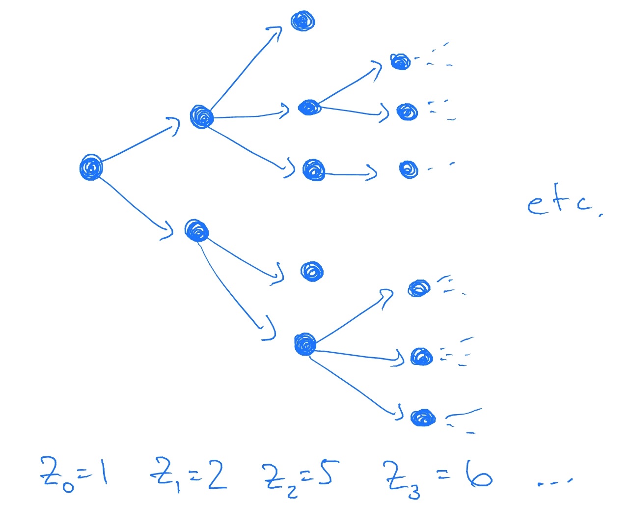
Each dot is a ‘parent’, which has a random number of child dots (indicated by arrows). Each parent choses how many children it will have independently of all else, by taking a random sample of \(G\). The BGW process is the process \(Z_n\), where \(Z_n\) is the number of dots in generation \(n\).
Formally, we define the BGW process as follows. Let \(X^n_i\), where \(n,i\ge 1\), be i.i.d. nonnegative integer-valued random variables with common distribution \(G\). Define a sequence \((Z_n)\) by \(Z_0=1\) and
\(\seteqnumber{0}{4.}{4}\)\begin{equation} \label {eq:gw_iterate} Z_{n+1} = \left \{ \begin{array}{ll} X^{n+1}_1 + \ldots + X^{n+1}_{Z_n}, & \mbox { if $Z_n>0$} \\ 0, & \mbox { if $Z_n=0$} \end {array} \right . \end{equation}
Then \(Z\) is the BGW process. The random variable \(X^n_i\) represents the number of children of the \(i^{th}\) parent in the \(n^{th}\) generation.
Note that if \(Z_n=0\) for some \(n\), then for all \(m>n\) we also have \(Z_m=0\).
-
Remark 4.3.1 The Bienaymé-Galton-Watson is commonly just called Galton-Watson process in the literature. It takes its name from Francis Galton (a statistician and social scientist) and Henry Watson (a mathematical physicist), who in 1874 were concerned that Victorian aristocratic surnames were becoming extinct. They tried to model how many children people had, which is also how many times a surname was passed on, per family. This allowed them to use the process \(Z_n\) to predict whether a surname would die out (i.e. if \(Z_n=0\) for some \(n\)) or become widespread (i.e. \(Z_n\to \infty \)). Unfortunately they made mistakes in their work, and in fact it turns out the French mathematician Irénée-Jules Bienaymé had entirely solved the question in 1845.
(Since then, the BGW process has found more important uses.)
Let us assume that \(G\in L^1\) and write \(\mu =\E [G]\). Let \(\mc {F}_n=\sigma (X^i_m\-i\in \N , m\leq n)\). In general, \(Z_n\) is not a martingale because
\(\seteqnumber{0}{4.}{5}\)\begin{align} \E [Z_{n+1}]&=\E \l [X^{n+1}_1 + \ldots + X^{n+1}_{Z_n}\r ]\notag \\ &=\E \l [\sum \limits _{k=1}^\infty \l (X^{n+1}_1 + \ldots + X^{n+1}_{k}\r )\1\{Z_n=k\}\r ]\notag \\ &=\sum \limits _{k=1}^\infty \E \l [\l (X^{n+1}_1 + \ldots + X^{n+1}_{k}\r )\1\{Z_n=k\}\r ]\notag \\ &=\sum \limits _{k=1}^\infty \E \l [\l (X^{n+1}_1 + \ldots + X^{n+1}_{k}\r )\r ]\E \l [\1\{Z_n=k\}\r ]\notag \\ &=\sum \limits _{k=1}^\infty \l (\E \l [X^{n+1}_1\r ] + \ldots + \E \l [X^{n+1}_{k}\r ]\r )\P \l [Z_n=k\r ]\notag \\ &=\sum \limits _{k=1}^\infty k\mu \P [Z_n=k]\notag \\ &=\mu \sum \limits _{k=1}^\infty k \P [Z_n=k]\notag \\ &=\mu \,\E [Z_n].\label {eq:br_exp} \end{align} Here, we use that the \(X^{n+1}_i\) are independent of \(\mc {F}_n\), but \(Z_n\) (and hence also \(\1\{Z_n=k\}\)) is \(\mc {F}_n\) measurable. We justify exchanging the infinite \(\sum \) and \(\E \) using the result of exercise (6.8).
From (4.6), Lemma 3.3.6 tells us that if \((M_n)\) is a martingale that \(\E [M_n]=\E [M_{n+1}]\). But, if \(\mu <1\) we see that \(\E [Z_{n+1}]<\E [Z_n]\) (downwards drift) and if \(\mu >1\) then \(\E [Z_{n+1}]>\E [Z_n]\) (upwards drift).
However, much like with the asymmetric random walk, we can compensate for the drift and obtain a martingale. More precisely, we will show that
\[M_n=\frac {Z_n}{\mu ^n}\]
is a martingale.
We have \(M_0=1\in m\mc {F}_0\), and if \(M_n\in \mc {F}_n\) then from (4.5) we have that \(M_{n+1}\in m\mc {F}_{n+1}\). Hence, by induction \(M_n\in \mc {F}_n\) for all \(n\in \N \). From (4.6), we have \(\E [Z_{n+1}]=\mu \E [Z_n]\) so as \(\E [Z_n]=\mu ^{n}\) for all \(n\). Hence \(\E [M_n]=1\) and \(M_n\in L^1\).
Lastly, we repeat the calculation that led to (4.6), but now with conditional expectation in place of \(\E \). The first few steps are essentially the same, and we obtain
\(\seteqnumber{0}{4.}{6}\)\begin{align*} \E [Z_{n+1}\|\F _n] &= \sum _{k=1}^\infty \E \l [\l (X^{n+1}_1 + \ldots + X^{n+1}_k\r )\1\{Z_n=k\} \|\F _n\r ] \\ &= \sum _{k=1}^\infty \1\{Z_n=k\} \E \l [X^{n+1}_1 + \ldots + X^{n+1}_k\|\F _n\r ]\\ &= \sum _{k=1}^\infty \1\{Z_n=k\} \E \l [X^{n+1}_1 + \ldots + X^{n+1}_k\r ]\\ &= \sum _{k=1}^\infty k \mu \1\{Z_n=k\}\\ &= \mu \sum _{k=1}^\infty k \1\{Z_n=k\}\\ &= \mu Z_n. \end{align*} Here we use that \(Z_n\) is \(\mc {F}_n\) measurable to take out what is known, and then use that \(X^{n+1}_i\) is independent of \(\mc {F}_n\). Hence, \(\E [M_{n+1}|\mc {F}_n]=M_n\), as required.