Stochastic Processes and Financial Mathematics
(part one)
Chapter A Solutions to exercises (part one)
Chapter 1
-
1.1 At time \(1\) we would have \(10(1+r)\) in cash and \(5\) units of stock. This gives the value of our assets at time \(1\) as \(10(1+r)+5S_1\).
-
-
(a) Assuming we don’t buy or sell anything at time \(0\), the value of our portfolio at time \(1\) will be \(x(1+r)+yS_1\), where \(S_1\) is as in the solution to 1.1. Since we need to be certain of paying off our debt, we should assume a worst case scenario for \(S_1\), that is \(S_1=sd\). So, we are certain to pay off our debt if and only if
\[x(1+r)+ysd \geq K.\]
-
(b) Since certainty requires that we cover the worst case scenario of our stock performance, and \(d<1+r\), our best strategy is to exchange all our assets for cash at time \(t=0\). This gives us \(x+ys\) in cash at time \(0\). At time \(1\) we would then have \((1+r)(x+ys)\) in cash at time \(0\) and could pay our debt providing that
\[(1+r)(x+ys) \geq K.\]
-
-
-
(a) We borrow \(s\) cash at time \(t=0\) and use it to buy one stock. Then wait until time \(t=1\), at which point we will a stock worth \(S_1\), where \(S_1\) is as in 1.1. We sell our stock, which gives us \(S_1\) in cash. Since \(S_1\geq sd>s(1+r)\), we repay or debt (plus interest) which costs us \(s(1+r)\). We then have
\[S_1-s(1+r)>0\]
in cash. This is an arbitrage.
-
(b) We perform the same strategy as in (a), but with the roles of cash an stock swapped: We borrow \(1\) stock at time \(t=0\) and then sell it for \(s\) in cash. Then wait until time \(t=1\), at which point we will have \(s(1+r)\) in cash. Since the price of a stock is now \(S_1\), where \(S_1\) is as in 1.1, and \(S_1\leq us<(1+r)s\), we now buy one stock costing \(S_1\) and repay the stockbroker, leaving us with
\[s(1+r)-S_1>0\]
in cash. This is an arbitrage.
-
-
1.4 We can calculate, using integration by parts, that
\(\seteqnumber{0}{A.}{0}\)\begin{align*} \E [X]=\int _{-\infty }^\infty x f_X(x)\,dx=\int _0^\infty x\lambda e^{-\lambda x}\,dx=\frac {1}{\lambda }. \end{align*} Similarly, we can calculate that
\[ \E [X^2]=\int _{-\infty }^\infty x^2 f_X(x)\,dx=\int _0^\infty x^2\lambda e^{-\lambda x}\,dx=\frac {2}{\lambda ^2} \]
This gives that
\[\var (X)=\E [X^2]-\E [X]^2=\frac {1}{\lambda ^2}.\]
-
1.5 We can calculate
\[\E [X_n]=0\cdot \P [X_n=0]+n^2\P [X_n=n^2]=\frac {n^2}{n}=n\to \infty \]
as \(n\to \infty \). Also,
\[\P [|X_n|>0]=\P [X_n=n^2]=\frac {1}{n}\to 0\]
as \(n\to \infty \).
-
1.6 We have
\(\seteqnumber{0}{A.}{0}\)\begin{align*} \P [Y\leq y] &=\P \l [\frac {X-\mu }{\sigma }\leq y\r ]\\ &=\P [X\leq \mu +y\sigma ]\\ &=\int _{-\infty }^{\mu +y\sigma }\frac {1}{\sqrt {2\pi \sigma ^2}}e^{-\frac {(x-\mu )^2}{2\sigma ^2}}\,dx. \end{align*} We want to turn the above integral into the distribution function of the standard normal. To do so, substitute \(z=\frac {x-\mu }{\sigma }\), and we obtain
\(\seteqnumber{0}{A.}{0}\)\begin{align*} \P [Y\leq y]&=\int _{-\infty }^y\frac {1}{\sqrt {2\pi \sigma ^2}}e^{-\frac {z^2}{2}}\sigma \,dz\\ &=\int _{-\infty }^y \frac {1}{\sqrt {2\pi }}e^{-\frac {z^2}{2}}\,dz. \end{align*} Hence, \(Y\) has the distribution function of \(N(0,1)\), which means \(Y\sim N(0,1)\).
-
1.7 For \(p\neq 1\),
\[\int _1^\infty x^{-p}\,dx = \l [\frac {x^{-p+1}}{-p+1}\r ]_{x=1}^\infty \]
and we obtain a finite answer only if \(-p+1<0\). When \(p=1\), we have
\[\int _1^\infty x^{-1}\,dx = \l [\log x\r ]_{x=1}^\infty =\infty ,\]
so we conclude that \(\int _1^\infty x^{-p}\,dx\) is finite if and only if \(p>1\).
-
1.8 As \(n\to \infty \),
-
• \(e^{-n}\to 0\) because \(e>1\).
-
• \(\sin \l (\frac {n\pi }{2}\r )\) oscillates through \(0,1,0,-1\) and does not converge.
-
• \(\frac {\cos (n\pi )}{n}\) converges to zero by the sandwich rule since \(|\frac {\cos (n\pi )}{n}|\leq \frac {1}{n}\to 0\).
-
• \(\sum \limits _{i=1}^n 2^{-i}=1-2^{-n}\) is a geometric series, and \(1-2^{-n}\to 1-0=1\).
-
• \(\sum \limits _{i=1}^n\frac {1}{i}\) tends to infinity, because
\[\overbrace {\frac 12}+\overbrace {\frac 13+\frac 14}+\overbrace {\frac 15+\frac 16+\frac 17+\frac 18}+\overbrace {\frac 19+\frac {1}{10}++\frac {1}{11}+\frac {1}{12}+\frac {1}{13}+\frac {1}{14}+\frac {1}{15}+\frac {1}{16}}+\ldots .\]
each term contained in a \(\overbrace {\cdot }\) is greater than or equal to \(\frac 12\).
-
-
1.9 Recall that \(\sum _{n=1}^\infty n^{-2}<\infty \). Define \(n_1=1\) and then
\[n_{r+1}=\inf \{k\in \N \-k>n_r\text { and }|x_k|\leq r^{-2}\}.\]
Then for all \(r\) we have \(|x_{n_r}|\leq r^{-2}\). Hence,
\[\sum \limits _{r=1}^\infty \l |x_{n_r}\r |\leq \sum \limits _{r=1}^\infty r^{-2}<\infty .\]
Chapter 2
-
2.1 The result of rolling a pair of dice can be written \(\omega =(\omega _1,\omega _2)\) where \(\omega _1,\omega _2\in \{1,2,3,4,5,6\}\). So a suitable \(\Omega \) would be
\[\Omega =\Big \{(\omega _1,\omega _2)\-\omega _1,\omega _2\in \{1,2,3,4,5,6\}\Big \}.\]
Of course other choices are possible too. Since our choice of \(\Omega \) is finite, a suitable \(\sigma \)-field is \(\mc {F}=\mc {P}(\Omega )\).
-
-
(a) Consider the case of \(\mc {F}\). We need to check the three properties in the definition of a \(\sigma \)-field.
-
1. We have \(\emptyset \in \mc {F}\) so the first property holds automatically.
-
2. For the second we check compliments: \(\Omega \sc \Omega =\emptyset \), \(\Omega \sc \{1\}=\{2,3\}\), \(\Omega \sc \{2,3\}=\{1\}\) and \(\Omega \sc \Omega =\emptyset \); in all cases we obtain an element of \(\mc {F}\).
-
3. For the third, we check unions. We have \(\{1\}\cup \{2,3\}=\Omega \). Including \(\emptyset \) into a union doesn’t change anything; including \(\Omega \) into a union results in \(\Omega \). This covers all possible cases, in each case resulting in an element of \(\mc {F}\).
So, \(\mc {F}\) is a \(\sigma \)-field. Since \(\mc {F}'\) is just \(\mc {F}\) with the roles of \(1\) and \(2\) swapped, by symmetry \(\mc {F}'\) is also a \(\sigma \)-field.
-
-
(b) We have \(\{1\}\in \mc {F}\cup \mc {F}'\) and \(\{2\}\in \mc {F}\cup \mc {F}'\), but \(\{1\}\cup \{2\}=\{1,2\}\) and \(\{1,2\}\notin \mc {F}\cup \mc {F}'\). Hence \(\mc {F}\cup \mc {F}'\) is not closed under unions; it fails property 3 of the definition of a \(\sigma \)-field.
However, \(\mc {F}\cap \mc {F}'\) is the intersection of two \(\sigma \)-fields, so is automatically itself a \(\sigma \)-field. (Alternatively, note that \(\mc {F}\cap \mc {F}'=\{\emptyset ,\Omega \}\), and check the definition.)
-
-
-
(a) Let \(A_m\) be the event that the sequence \((X_n)\) contains precisely \(m\) heads. Let \(A_{m,k}\) be the event that we see precisely \(m\) heads during the first \(k\) tosses and, from then on, only tails. Then,
\(\seteqnumber{0}{A.}{0}\)\begin{align*} \P [A_{m,k}] &=\P [m\text { heads in }X_1,\ldots ,X_k,\text { no heads in }X_{k+1},X_{k+2},\ldots ]\\ &=\P [m\text { heads in }X_1,\ldots ,X_k,]\,\P [\text { no heads in }X_{k+1},X_{k+2},\ldots ]\\ &=\P [m\text { heads in }X_1,\ldots ,X_k,]\times 0\\ &=0. \end{align*} If \(A_m\) occurs then at least one of \(A_{m,1},A_{m,2},\ldots \) occurs. Hence,
\[\P [A_m]\leq \sum \limits _{k=0}^\infty \P [A_{m,k}]=0\]
.
-
(b) Let \(A\) be the event that the sequence \((X_n)\) contains finitely many heads. Then, if \(A\) occurs, precisely one of \(A_1,A_2,\ldots \) occurs. Hence,
\[\P [A]=\sum \limits _{m=0}^\infty \P [A_m]=0.\]
That is, the probability of having only finite many heads is zero. Hence, almost surely, the sequence \((X_n)\) contains infinitely many heads.
By symmetry (exchange the roles of heads and tails) almost surely the sequence \((X_n)\) also contains infinitely many tails.
-
-
-
(a) \(\F _1\) contains the information of whether a \(6\) was rolled.
-
(b) \(\F _2\) gives the information of which value was rolled if a \(1\), \(2\) or \(3\) was rolled, but if the roll was in \(\{4,5,6\}\) then \(\F _1\) cannot tell the difference between these values.
-
(c) \(\F _3\) contains the information of which of the sets \(\{1,2\}\), \(\{3,4\}\) and \(\{5,6\}\) contains the value rolled, but gives no more information than that.
-
-
-
(a) The values taken by \(X_1\) are
\[X_1(\omega )= \begin {cases} 0 & \text { if }\omega =3,\\ 1 & \text { if }\omega =2,4,\\ 4 & \text { if }\omega =1,5.\\ \end {cases} \]
Hence, the pre-images are \(X_1^{-1}(0)=\{3\}\), \(X_1^{-1}(1)=\{2,4\}\) and \(X_1^{-1}(4)=\{1,5\}\). These are all elements of \(\G _1\), so \(X_1\in m\G _1\). However, they are not all elements of \(\G _2\) (in fact, none of them are!) so \(X_1\notin m\G _2\).
-
(b) Define
\[X_2(\omega )= \begin {cases} 0 & \text { if }\omega =1,2,\\ 1 & \text { otherwise}. \end {cases} \]
Then the pre-images are \(X_2^{-1}(0)=\{1,2\}\) and \(X_2^{-1}(1)=\{3,4,5\}\). Hence \(X_2\in m\G _2\).
It isn’t possible to use unions/intersections/complements to make the set \(\{3,4,5\}\) out of \(\{1,5\},\{2,4\},\{3\}\) (one way to see this is note that as soon as we tried to include \(5\) we would also have to include \(1\), meaning that we can’t make \(\{3,4,5\}\)). Hence \(X_2\notin m\G _1\).
-
-
2.6 We have \(X(TT)=0\), \(X(HT)=X(TH)=1\) and \(X(HH)=2\). This gives
\[\sigma (X)=\Big \{\emptyset , \{TT\}, \{TH, HT\}, \{HH\}, \{TT, TH, HT\}, \{TT, HH\}, \{TH, HT, HH\}, \Omega \Big \}.\]
To work this out, you could note that \(X^{-1}(i)\) must be in \(\sigma (X)\) for \(i=0,1,2\), then also include \(\emptyset \) and \(\Omega \), then keep adding unions and complements of the events until find you have added them all. (Of course, this only works because \(\sigma (X)\) is finite!)
-
2.7 Since sums, divisions and products of random variables are random variables, \(X^2+1\) is a random variable. Since \(X^2+1\) is non-zero, we have that \(\frac {1}{X^2+1}\) is a random variable, and using products again, \(\frac {X}{X^2+1}\) is a random variable.
For \(\sin (X)\), recall that for any \(x\in \R \) we have
\[\sin (x)=\sum _{n=0}^\infty \frac {(-1)^n}{(2n+1)!}x^{2n+1}.\]
Since \(X\) is a random variable so is \(\frac {(-1)^n}{(2n+1)!}X^{2n+1}\). Since limits of random variables are also random variables, so is
\[\sin X=\lim \limits _{N\to \infty }\sum _{n=0}^N\frac {(-1)^n}{(2n+1)!}X^{2n+1}.\]
-
2.8 Since \(X\geq 0\) we have \(\E [X^p]=\E [|X|^p]\) for all \(p\).
\[\E [X]=\int _1^\infty x^12x^{-3}\,dx=2\int _1^\infty x^{-2}\,dx=2\l [\frac {x^{-1}}{-1}\r ]_1^\infty =2<\infty \]
so \(X\in L^1\), but
\[\E [X^2]=\int _1^\infty x^22x^{-3}\,dx=2\int _1^\infty x^{-1}\,dx=2\l [\log x\r ]_1^\infty =\infty \]
so \(X\notin L^2\).
-
2.9 Let \(1\leq p\leq q<\infty \) and \(X\in L^q\). Our plan is to generalize the argument that we used to prove (2.7).
First, we condition to see that
\[|X|^p=|X|^p\1\{|X|\leq 1\}+|X|^p\1\{|X|>1\}.\]
Hence,
\(\seteqnumber{0}{A.}{0}\)\begin{align*} \E [|X|^p] &=\E \l [|X|^p\1\{|X|\leq 1\}+|X|^p\1\{|X|>1\}\r ]\\ &\leq \E \l [1+|X|^q\r ]\\ &=1+\E |X|^q]<\infty \end{align*} Here we use that, if \(|X|\leq 1\) then \(|X|^p\leq 1\), and if \(|X|>1\) then since \(p\leq q\) we have \(|X|^p<|X|^q\). So \(X\in L^p\).
-
2.10 First, we condition to see that
\(\seteqnumber{0}{A.}{0}\)\begin{equation} \label {eq:markovs_pre} X=X\1_{\{X< a\}}+X\1_{\{X\geq a\}}. \end{equation}
From (A.1) since \(X\geq 0\) we have
\(\seteqnumber{0}{A.}{1}\)\begin{align*} X &\geq X\1_{\{X\geq a\}}\\ &\geq a\1\{X\geq a\}. \end{align*} This second inequality follows by looking at two cases: if \(X<a\) then both sides are zero, but if \(X\geq a\) then we can use that \(X\geq a\). Using monotonicity of \(\E \), we then have
\[\E [X]\geq \E [a\1_{\{X\geq a\}}]=a\E [1_{\{X\geq a\}}]=a\P [X\geq a].\]
Dividing through by \(a\) finishes the proof.
This result is known as Markov’s inequality.
-
2.11 Since \(X\geq 0\), Markov’s inequality (from 2.10) gives us that
\[\P [X\geq a]\leq \frac {1}{a}\E [X]=0\]
for any \(a>0\). Hence,
\(\seteqnumber{0}{A.}{1}\)\begin{align*} \P [X>0]&=\P [X>1]+\P [1\geq X>0]\\ &=\P [X>1]+\P \l [\bigcup \limits _{n=1}^\infty \l \{\tfrac {1}{n}\geq X>\tfrac {1}{n+1}\r \}\r ]\\ &=\P [X>1]+\sum \limits _{n=1}^\infty \P \l [\tfrac {1}{n}\geq X>\tfrac {1}{n+1}\r ]\\ &\leq \P [X\geq 1]+\sum \limits _{n=1}^\infty \P \l [X>\tfrac {1}{n+1}\r ]\\ &=0. \end{align*}
Chapter 3
-
3.1 We have \(S_2=X_1+X_2\) so
\(\seteqnumber{0}{A.}{1}\)\begin{align*} \E [S_2\|\sigma (X_1)] &=\E [X_1\|\sigma (X_1)]+\E [X_2\|\sigma (X_1)]\\ &=X_1+\E [X_2]\\ &=X_1. \end{align*} Here, we use the linearity of conditional expectation, followed by the fact that \(X_1\) is \(\sigma (X_1)\) measurable and \(X_2\) is independent of \(\sigma (X_1)\) with \(\E [X_2]=0\).
Secondly, \(S_2^2=X_1^2+2X_1X_2+X_2^2\) so
\(\seteqnumber{0}{A.}{1}\)\begin{align*} \E [S_2^2] &=\E [X_1^2\|\sigma (X_1)]+2\E [X_1X_2\|\sigma (X_1)]+\E [X_2^2\|\sigma (X_1)]\\ &=X_1^2+2X_1\E [X_2\|\sigma (X_1)]+\E [X_2^2]\\ &=X_1^2+1 \end{align*} Here, we again use linearity of conditional expectation to deduce the first line. To deduce the second line, we use that \(X_1^2\) and \(X_1\) are \(\sigma (X_1)\) measurable (using the taking out what is known rule for the middle term), whereas \(X_2\) is independent of \(\sigma (X_1)\). The final line comes from \(\E [X_2\|\sigma (X_1)]=0\) (which we already knew from above) and that \(\E [X_2^2]=1\).
-
3.2 For \(i\leq n\), we have \(X_i\in m\mc {F}_n\), so \(S_n=X_1+X_2+\ldots +X_n\) is also \(\mc {F}_n\) measurable. For each \(i\) we have \(|X_i|\leq 2\) so \(|S_n|\leq 2n\), hence \(S_n\in L^1\). Lastly,
\(\seteqnumber{0}{A.}{1}\)\begin{align*} \E [S_{n+1}\|\mc {F}_n] &=\E [X_1+\ldots +X_n\|\mc {F}_n]+\E [X_{n+1}\|\mc {F}_n]\\ &=(X_1+\ldots +X_n) + \E [X_{n+1}]\\ &=S_n. \end{align*} Here, we use linearity of conditional expectation in the first line. To deduce the second, we use that \(X_i\in m\mc {F}_n\) for \(i\leq n\) and that \(X_{n+1}\) is independent of \(\mc {F_n}\) in the second. For the final line we note that \(\E [X_{n+1}]=\frac 132+\frac 23(-1)=0\).
-
-
(a) Since \(X_i\in m\mc {F}_n\) for all \(i\leq n\), we have \(M_n=X_1X_2\ldots X_n\in m\mc {F}_n\). Since \(|X_i|\leq c\) for all \(i\), we have \(|M_n|\leq c^n<\infty \), so \(M_n\) is bounded and hence \(M_n\in L^1\) for all \(n\). Lastly,
\(\seteqnumber{0}{A.}{1}\)\begin{align*} \E [M_{n+1}\|\mc {F}_n] &=\E [X_1X_2\ldots X_nX_{n+1}\|\mc {F}_n]\\ &=X_1\ldots X_n\E [X_{n+1}\|\mc {F}_n]\\ &=X_1\ldots X_n\E [X_{n+1}]\\ &=X_1\ldots X_n\\ &=M_n. \end{align*} Here, to deduce the second line we use that \(X_i\in m\mc {F}_n\) for \(i\leq n\). To deduce the third line we use that \(X_{n+1}\) is independent of \(\mc {F}_n\) and then to deduce the forth line we use that \(\E [X_{n+1}]=1\).
-
(b) By definition of conditional expectation (Theorem 3.1.1), we have \(M_n\in L^1\) and \(M_n\in m\mc {G}_n\) for all \(n\). It remains only to check that
\(\seteqnumber{0}{A.}{1}\)\begin{align*} \E [M_{n+1}\|\mc {G}_n] &=\E [\E [Z\|\mc {G}_{n+1}]\|\mc {G}_n]\\ &=\E [Z\|\mc {G}_n]\\ &=M_n. \end{align*} Here, to get from the first to the second line we use the tower property.
-
-
3.4 Note that the first and second conditions in Definition 3.3.3 are the same for super/sub-martingales as for martingales. Hence, \(M\) satisfies these conditions. For the third condition, we have that \(\E [M_{n+1}\|\mc {F}_n]\leq M_n\) (because \(M\) is a supermartingale) and \(\E [M_{n+1}\|\mc {F}_n]\geq M_n\) (because \(M\) is a submartingale. Hence \(\E [M_{n+1}\|\mc {F}_n]=M_n\), so \(M\) is a martingale.
-
-
(a) If \(m=n\) then \(\E [M_n\|\mc {F}_n]=M_n\) because \(M_n\) is \(\mc {F}_n\) measurable. For \(m>n\), we have
\[\E [M_m|\mc {F}_n]=\E [\E [M_m\|\mc {F}_{m-1}]\|\mc {F}_n]=\E [M_{m-1}\|\mc {F}_n].\]
Here we use the tower property to deduce the first equality (note that \(m-1\geq n\) so \(\mc {F}_{m-1}\supseteq \mc {F}_n\)) and the fact that \((M_n)\) is a martingale to deduce the second inequality (i.e. \(\E [M_{m}\|\mc {F}_{m-1}]=M_{m-1}\)). Iterating, from \(m,m-1\ldots ,n+1\) we obtain that
\[\E [M_m\|\mc {F}_n]=\E [M_{n+1}\|\mc {F}_n]\]
and the martingale property then gives that this is equal to \(M_n\), as required.
-
(b) If \((M_n)\) is a submartingale then \(\E [M_m\|\mc {F}_n]\geq M_n\), whereas if \((M_n)\) is a supermartingale then \(\E [M_m\|\mc {F}_n]\leq M_n\).
-
-
3.6 We have \((M_{n+1}-M_n)^2=M_{n+1}^2-2M_{n+1}M_n+M_n^2\) so
\(\seteqnumber{0}{A.}{1}\)\begin{align*} \E \l [(M_{n+1}-M_n)^2\|\mc {F}_n\r ] &=\E [M_{n+1}^2\|\mc {F}_n]-2\E [M_{n+1}M_n\|\mc {F}_n]+\E [M_n^2\|\mc {F}_n]\\ &=\E [M_{n+1}^2\|\mc {F}_n]-2M_n\E [M_{n+1}\|\mc {F}_n]+M_n^2\\ &=\E [M_{n+1}^2\|\mc {F}_n]-2M_n^2+M_n^2\\ &=\E [M_{n+1}^2\|\mc {F}_n]-M_n^2 \end{align*} as required. Here, we use the taking out what is known rule (since \(M_n\in m\mc {F}_n\)) and the martingale property of \((M_n)\).
It follows that \(\E [M_{n+1}^2\|\mc {F}_n]-M_n^2=\E [(M_{n+1}-M_n)^2\|\mc {F}_n]\geq 0\). We have \(M_n^2\in m\mc {F}_n\) and since \(M_n\in L^2\) we have \(M_n^2\in L^1\). Hence \((M_n^2)\) is a submartingale.
-
3.7 Using that \(\E [X_{n+1}\|\mc {F}_n]=aX_n+bX_{n-1}\) we can calculate
\[\E [S_{n+1}\|\mc {F}_n]=\E [\alpha X_{n+1}+X_{n}\|\mc {F}_n]=\alpha (aX_n+bX_{n-1})+X_n=(\alpha a+1)X_n+\alpha b X_{n-1}.\]
We want this to be equal to \(S_n\), and \(S_n=\alpha X_n+X_{n-1}\). So we need
\[\alpha a+1=\alpha \hspace {1pc}\text { and }\hspace {1pc}\alpha b = 1.\]
Hence, \(\alpha =\frac {1}{b}\) is our choice. It is then easy to check that
\[\E [S_{n+1}\|\mc {F}_n]=\tfrac {1}{b}(aX_n+bX_{n-1})+X_n=(\tfrac {a}{b}+1)X_n+X_{n-1}=\tfrac {1}{b}X_n+X_{n-1}=S_n\]
and thus \(S_n\) is a martingale, as required.
-
3.8 Note that
\[\E [X_1\|\sigma (S_n)]=\E [X_2\|\sigma (S_n)]=\ldots =\E [X_n\|\sigma (S_n)]\]
is constant, by symmetry (i.e. permuting the \(X_1,X_2,\ldots ,X_n\) does not change the distribution of \(S_n\)). Hence, if we set \(\E [X_i\|\sigma (S_n)]=\alpha \) then
\(\seteqnumber{0}{A.}{1}\)\begin{align*} n\alpha =\sum \limits _{i=1}^n\E [X_i\|\sigma (S_n)]=\E \l [\sum \limits _{i=1}^n X_i\,\Big |\,\sigma (S_n)\r ]=\E [S_n\|\sigma (S_n)]=S_n. \end{align*} Here we use the linearity of conditional expectation and the fact that \(S_n\) is \(\sigma (S_n)\) measurable. Hence,
\[\alpha =\E [X_1\|\sigma (S_n)]=\frac {S_n}{n}.\]
Chapter 4
-
4.1 Since \(Z_n=e^{S_n}\) and \(S_n\in m\mc {F}_n\), also \(Z_n\in m\mc {F}_n\). Since \(|S_n|\leq n\), we have \(|e^{S_n}|\leq e^n<\infty \), so \(Z_n\) is bounded and hence \(Z_n\in L^1\). Hence also \(M_n\in m\mc {F}_n\) and \(M_n\in L^1\).
Lastly,
\(\seteqnumber{0}{A.}{1}\)\begin{align*} \E [e^{S_{n+1}}|\mc {F}_n] &= \E [e^{X_{n+1}}e^{S_n}\|\mc {F}_n] \\ &= e^{S_n}\E [e^{X_{n+1}}\|\mc {F}_n] \\ &= e^{S_n}\E [e^{X_{n+1}}] \\ &= e^{S_n}\l (\tfrac 12 e+\tfrac 12 e^{-1}\r )\\ &= e^{S_n}\frac {e+\frac {1}{e}}{2}. \end{align*} Here, we use the taking out what is known rule and the fact that \(X_{n+1}\) (and hence also \(e^{X_{n+1}}\)) is independent of \(\mc {F}_n\). We also calculate the expectation of the discrete random variable \(X_{n+1}\), using that \(\P [X_{n+1}=1]=\P [X_{n+1}=-1]=\frac 12\). This gives us that
\(\seteqnumber{0}{A.}{1}\)\begin{align*} \E [M_{n+1}\|\mc {F}_n]&= M_n\\ \E [Z_{n+1}\|\mc {F}_n]&\geq Z_n \end{align*} where to deduce the last line we use that \(\frac {e+\frac {1}{e}}{2}>1\). Thus \(M_n\) is a martingale and \(Z_n\) is a submartingale.
-
4.2 Since \(X_i\in m\mc {F}_n\) for all \(i\leq n\), we have \(M_n\in m\mc {F}_n\). We have \(|X_i|\leq 1\) so \(|S_n|\leq n\) and \(|M_n|\leq \max \{(q/p)^n, (q/p)^{-n}\}=(q/p)^{-n}\) (note \(p>q\)), which implies that \(S_n\in L^1\) and \(M_n\in L^1\) for all \(n\).
We have
\(\seteqnumber{0}{A.}{1}\)\begin{align*} \E [S_{n+1}\|\mc {F}_n] &=\E [S_{n}+X_{n+1}\|\mc {F}_n]\\ &=S_n+\E [X_{n+1}\|\mc {F}_n]\\ &=S_n+\E [X_{n+1}]\\ &>S_n. \end{align*} Here we use the taking out what is known rule, followed by the fact that \(X_{n+1}\) is independent of \(\mc {F}_{n}\) and the relationship between conditional expectation and independence. To deduce the final step we use that \(\E [X_{n+1}]=p(1)+q(-1)=p-q>0\). Therefore, we have \(\E [S_{n+1}\|\mc {F}_n]\geq S_n\), which means that \(S_n\) is a submartingale.
We now look at \(M_n\). We have
\(\seteqnumber{0}{A.}{1}\)\begin{align*} \E [M_{n+1}|\mc {F}_n]&=(q/p)^{S_n}\E [(q/p)^{X_{n+1}}|\mc {F}_n]\\ &=(q/p)^{S_n}\E [(q/p)^{X_{n+1}}]\\ &=(q/p)^{S_n}=M_n. \end{align*} Here we use the taking out what is known rule, followed by the fact that \(X_{n+1}\) is independent of \(\mc {F}_{n}\) and the relationship between conditional expectation and independence. To deduce the final step we use that
\[\E \l [(q/p)^{X_{n+1}}\r ]=p(q/p)^1+q(q/p)^{-1}=p+q=1.\]
-
4.3 Since \(X_i\in \mc {F}_n\) for all \(i\leq n\) we have \(S_n\in m\mc {F}_n\) where \(\mc {F}_n=\sigma (X_1,\ldots , X_n)\). Further, if we set \(m=\max (|a|,|b|)\) then \(|S_n|\leq nm\) so \(S_n\in L^1\).
We have
\(\seteqnumber{0}{A.}{1}\)\begin{align*} \E [S_{n+1}\|\mc {F}_n] &=\E [S_n+X_{n+1}\|\mc {F}_n]\\ &=S_n+\E [X_{n+1}\|\mc {F}_n]\\ &=S_n+\E [X_{n+1}]\\ &=S_n+ap_a-bp_b \end{align*} where \(p_b=1-p_a\). Therefore, \(S_n\) is a martingale if and only if \(ap_a=bp_b\).
-
4.4 Clearly \(S_n\in m\mc {F}_n\) (recall that, by default, we take \((\mc {F}_n)\) to be the generated filtration of \((S_n)\)) hence \(S_n^2\in m\mc {F}_n\) and \(S_n^2-n\in \mc {F}_n\). We have \(|S_n|leq n\) so \(\E [|S_n^2-n]\leq \E [S_n^2]+\E [n]=2n\) by the triangle law and monotonicity of expectation, hence \(S_n^2-n\in \ L^1\). Similarly \(S_n^2\in L^2\),
We have
\(\seteqnumber{0}{A.}{1}\)\begin{align*} \E [S_{n+1}^2-(n+1)\|\mc {F}_n] &= \E [(X_{n+1}+S_n)^2-(n+1)\|\mc {F}_n] \\ &= \E [X_{n+1}^2\|\mc {F}_n]+2\E [S_nX_{n+1}\|\mc {F}_n]+\E [S_n^2\|\mc {F}_n] - (n+1)\\ &= \E [X_{n+1}^2]+2S_n\E [X_{n+1}]+S_n^2 - (n+1)\\ &= 1 + 2S_n(0)+S_n^2 - (n+1) \\ &= S_n^2-n \end{align*} Here, the second line follows by linearity. The third line follows by the taking out what is known rule and the independence rule, using that \(X_{n+1}\) is independent of \(\mc {F}_n\), whilst \(S_n\in m\mc {F}_n\). The fourth line follows because \(X_{n+1}^2=1\) and \(\E [X_{n+1}]=\frac 12(1)+\frac 12(-1)=0\). Hence \(M_n=S_n^2-n\) is a martingale.
Subtracting \(n\) from both sides, we obtain \(\E [S_{n+1}^2\|\mc {F}_n]=S_n^2+1\). Hence \((S_n^2)\) is a submartingale.
-
4.5 The natural filtration is \(\mc {F}_n=\sigma (X_1,\ldots ,X_n)\). We can write
\[S_{n+1}=\1\{S_n=0\}+\1\{S_n\neq 0\}(S_n+X_{n+1}).\]
Hence, if \(S_n\in m\mc {F}_n\) then \(S_{n+1}\in m\mc {F}_{n+1}\). Since \(S_1=X_1\in m\mc {F}_n\), a trivial induction shows that \(S_n\in m\mc {F}_n\) for all \(n\). hence, \(L_n\in m\mc {F}_n\) and also \(S_n-L_n\in m\mc {F}_n\).
We have \(-n\leq S_n-L_n \leq n+1\) (because the walk is reflected at zero and can increase by at most \(1\) in each time step) so \(S_{n}-L_n\) is bounded and hence \(S_n-L_n\in L^1\).
Lastly,
\(\seteqnumber{0}{A.}{1}\)\begin{align} \E [S_{n+1}|\mc {F}_n] &=\E [\1\{S_n=0\}+\1\{S_n\neq 0\}(S_n+X_{n+1})\|\mc {F}_n]\notag \\ &=\1\{S_n=0\}+\1\{S_n\neq 0\}(S_n+\E \l [X_{n+1}|\mc {F}_n\r ])\notag \\ &=\1\{S_n=0\}+\1\{S_n\neq 0\}S_n\notag \\ &=\1\{S_n=0\}+S_n.\label {eq:SnLnpre} \end{align} Here we use linearity and the taking out what is known \((S_n\in m\mc {F}_n)\) rule, as well as that \(X_{n+1}\) is independent of \(\mc {F}_n\). Hence,
\(\seteqnumber{0}{A.}{2}\)\begin{align*} \E [S_{n+1}-L_{n+1}\|\mc {F}_n] &=\E \l [S_{n+1}-\sum \limits _{i=0}^n \1\{S_i=0\}\,\Bigg |\,\mc {F}_n\r ]\\ &=S_{n}+\1\{S_n=0\}-\sum \limits _{i=0}^n \1\{S_i=0\}\\ &=S_n-\sum \limits _{i=0}^{n-1} \1\{S_i=0\}\\ &=S_n-L_n \end{align*} Here we use (A.2) to deduce the second line, as well as taking out what is known. Hence, \(S_n-L_n\) is a martingale.
-
4.6 Let \(B_n\) be number of red balls in the urn at time \(n\) (i.e. after the \(n^{th}\) draw is complete). Then, the proportion of red balls in the urn just after the \(n^{th}\) step is
\[M_n=\frac {B_n}{n+3}.\]
Essentially the same argument as for the two colour urn of Section 4.2 shows that \(M_n\) is adapted to the natural filtration and also in \(L^1\). We have
\(\seteqnumber{0}{A.}{2}\)\begin{align*} \E [M_{n+1}\|\mc {F}_n] &=\E \l [M_{n+1}\1_{\{(n+1)^{th}\text { draw is red}\}}+M_{n+1}\1_{\{(n+1)^{th}\text { draw is not red}\}}\,\Big |\,\mc {F}_n\r ]\\ &=\E \l [\frac {B_n+1}{n+4}\1_{\{(n+1)^{th}\text { draw is red}\}}+\frac {B_n}{n+4}\1_{\{(n+1)^{th}\text { draw is not red}\}}\,\Big |\,\mc {F}_n\r ]\\ &=\frac {B_n+1}{n+4}\E \l [\1_{\{(n+1)^{th}\text { draw is red}\}}\,\Big |\,\mc {F}_n\r ]+\frac {B_n}{n+4}\E \l [\1_{\{(n+1)^{th}\text { draw is not red}\}}\,\Big |\,\mc {F}_n\r ]\\ &=\frac {B_n+1}{n+4}\frac {B_n}{n+3}+\frac {B_n}{n+4}\l (1-\frac {B_n}{n+3}\r )\\ &=\frac {B_n(n+4)}{(n+3)(n+4)}\\ &=M_n. \end{align*} Hence \((M_n)\) is a martingale.
-
4.7 By the result of 3.6, \(S_n^2\) is a submartingale.
-
(i) \(M_n=S_n^2+n\) is \(\mc {F}_n\) measurable (because \(S_n\in m\mc {F}_n\)) and since \(|S_n|\leq n\) we have \(|M_n|\leq n^2+n<\infty \), so \(M_n\in L^1\). Further, using the submartingale property of \(S_n^2\),
\[\E [S_{n+1}^2+n+1\|\mc {F}_n]=\E [S_{n+1}^2\|\mc {F}_n]+n+1\geq S_n^2+n\]
so \(M_n\) is a submartingale. But \(\E [M_1]=2\neq 0=\E [M_0]\), so (by Lemma 3.3.6) we have that \((M_n)\) is not a martingale.
-
(ii) We have shown in Section 4.1 that \((S_n)\) is a martingale, and in Exercise 4.4 that \(M_n=S_n^2-n\) is a martingale. Hence \(S_n^2-n+S_n\in \mc {F}_n\) and \(\E [|S_n^2+S_n-n|]\leq \E [|S_n^2-n|]+\E [|S_n|]<\infty \) by the triangle law, so also \(S_n^2+S_n-n\in L^1\). Also,
\(\seteqnumber{0}{A.}{2}\)\begin{align*} \E [S_{n+1}^2+S_{n+1}-(n+1)\|\mc {F}_n] &= \E [S_{n+1}^2-(n+1)\|\mc {F}_n]+\E [S_{n+1}\|\mc {F}_n] \\ &= S_n^2-n+S_n \end{align*} as required. To deduce the second line we use the martingale properties of \((S_n)\) and \((M_n)\). As all martingales are submartingales, this case is also a submartingale.
More generally, the sum of two martingales is always a martingale. The same is true for submartingales and also for supermartingales.
-
(iii) \(M_n=\frac {S_n}{n}\) is \(\mc {F}_n\) measurable (because \(S_n\in m\mc {F}_n\)) and since \(|S_n|\leq n\) we have \(|S_n|\leq 1\), so \(M_n\in L^1\). Since \(S_n\) is a martingale, we have
\[\E \l [\frac {S_{n+1}}{n+1}\,\Big {|}\,\mc {F}_n\r ]=\frac {1}{n+1}\E [S_{n+1}|\mc {F}_n]=\frac {S_n}{n+1}\neq \frac {S_n}{n}.\]
Hence \(M_n=\frac {S_n}{n}\) is not a martingale. Also, since \(S_n\) may be both positive or negative, we do not have \(\frac {S_n}{n+1}\geq \frac {S_n}{n}\), so \(S_n\) is also not a submartingale.
-
-
4.8 We showed that \(S_n^2-n\) was a martingale in 4.7. We try to mimic that calculation and find out what goes wrong in the cubic case. So, we look at
\(\seteqnumber{0}{A.}{2}\)\begin{align*} \E [(S_{n+1}-S_n)^3\|\mc {F}_n] &=\E [S_{n+1}^3\|\mc {F}_n]-3S_n\E [S_{n+1}^2\|\mc {F}_n]+3S_n^2\E [S_{n+1}\|\mc {F}_n]-\E [S_n^3\|\mc {F}_n]\\ &=\E [S_{n+1}^3\|\mc {F}_n]-3S_n(S_n^2+1)+3S_n^2S_n-S_n^3\\ &=\E [S_{n+1}^3\|\mc {F}_n]-S_n^3-3S_n. \end{align*} Here we use linearity, taking out what is known and that fact that \(\E [S_{n+1}^2\|\mc {F}_n]=S_n^2+1\) (from 4.7). However, also \(S_{n+1}-S_n=X_{n+1}\), so
\(\seteqnumber{0}{A.}{2}\)\begin{align*} \E [(S_{n+1}-S_n)^3\|\mc {F}_n] &=\E [X_{n+1}^3\|\mc {F}_n]\\ &=\E [X_{n+1}^3]\\ &=0. \end{align*} because \(X_{n+1}\) is independent of \(\mc {F}_n\) and \(X_{n+1}^3=X_n\) (it takes values only \(1\) or \(-1\)) so \(\E [X_{n+1}^3]=0\). Putting these two calculations together, we have
\(\seteqnumber{0}{A.}{2}\)\begin{equation} \label {eq:sn3_mart} \E [S_{n+1}^3\|\mc {F}_n]=S_n^3+3S_n. \end{equation}
Suppose (aiming for a contradiction) that there is a deterministic function \(f:\N \to \R \) such that \(S_n^3-f(n)\) is a martingale. Then
\[\E [S_{n+1}^3-f(n+1)\|\mc {F}_n]=S_n^3-f(n).\]
Combining the above equation with (A.3) gives
\[f(n+1)-f(n)=3S_n\]
but this is impossible because \(S_n\) is not deterministic. Thus we reach a contradiction; no such function \(f\) exists.
Chapter 5
-
5.1 The value of the portfolio \((1,3)\) at time \(1\) will be
\[1(1+r)+3S_1=(1+r)+3S_1\]
where \(S_1\) is a random variable with \(\P [S_1=su]=p_u\) and \(\P [S_1=sd]=p_d\).
-
-
(a) We need a portfolio \(h=(x,y)\) such that \(V^h_1=\Phi (S_1)=1\), so we need that
\(\seteqnumber{0}{A.}{3}\)\begin{align*} x(1+r)+ysu&=1\\ x(1+r)+ysd&=1. \end{align*} Solving this pair of linear equations gives \(x=\frac {1}{1+r}\) and \(y=0\). So our replicating portfolio consists simply of \(\frac {1}{1+r}\) cash and no stock.
Hence, the value of this contingent claim at time \(0\) is \(x+sy=\frac {1}{1+r}\).
-
(b) Now we need that
\(\seteqnumber{0}{A.}{3}\)\begin{align*} x(1+r)+ysu=3\\ x(1+r)+ysd=1. \end{align*} Which has solution \(x=\frac {1}{1+r}\l (3-\frac {2su}{su-sd}\r )\) and \(y=\frac {2}{s(u-d)}\).
Hence, the value of this contingent claim at time \(0\) is \(x+sy=\frac {1}{1+r}\l (3-\frac {2su}{su-sd}\r )+\frac {2}{u-d}\).
-
-
-
(a) If we buy two units of stock, at time \(1\), for a price \(K\) then our contingent claim is \(\Phi (S_1)=2S_1-2K\).
-
(b) In a European put option, with strike price \(K\in (sd,su)\), we have the option to sell a single unit of stock for strike price \(K\). It is advantageous to us to do so only if \(K>S_1\), so
\(\seteqnumber{0}{A.}{3}\)\begin{equation} \label {eq:eu_put_contingent} \Phi (S_1)=\begin{cases} 0 & \text { if }S_1=su,\\ K-S_1 & \text { if }S_1=sd. \end {cases} =\max (K-S_1, 0) \end{equation}
-
(c) We \(S_1=su\) we sell a unit of stock for strike price \(K\) and otherwise do nothing. So our contingent claim is
\[\Phi (S_1)=\begin {cases} K-S_1 & \text { if }S_1=su,\\ 0 & \text { if }S_1=sd. \end {cases} \]
-
(d) Holding both the contracts in (b) and (c) at once, means that in both \(S_1=su\) and \(S-1=sd\), we end up selling a single unit of stock for a fixed price \(K\). Our contingent claim for doing so is \(\Phi (S_1)=K-S_1\).
-
-
-
(a) The contingent claims for the call and put options respectively are \(\max (S_1-K,0)\) from (5.6) and \(\max (K-S_1,0)\) from (A.4). Using the risk neutral valuation formula from Proposition 5.2.6 we have
\[\Pi ^{call}_0=\frac {1}{1+r}\E ^\Q \l [\max (S_1-K,0)\r ],\quad \Pi ^{put}_0=\frac {1}{1+r}\E ^\Q \l [\max (K-S_1,0)\r ].\]
-
(b) Hence,
\(\seteqnumber{0}{A.}{4}\)\begin{align*} \Pi ^{call}_0-\Pi ^{put}_0&=\frac {1}{1+r}\E ^\Q \l [\max (S_1-K,0)-\max (K-S_1,0)\r ]\\ &=\frac {1}{1+r}\E ^\Q \l [\max (S_1-K,0)+\min (S_1-K,0)\r ]\\ &=\frac {1}{1+r}\E ^\Q \l [S_1-K\r ]\\ &=\frac {1}{1+r}\l (\E ^\Q \l [S_1\r ]-K\r )\\ \end{align*} By (5.4) (or you can use Proposition 5.2.6 again) we have \(\frac {1}{1+r}\E ^\Q \l [S_1\r ]=S_0=s\), so we obtain
\[\Pi ^{call}_0-\Pi ^{put}_0=s-\frac {K}{1+r}.\]
-
-
5.5 In the binomial model, the contingent claim of a European call option with strike price \(K\) is \(\Phi (S_T)=\max (S_T-K)\).
-
5.6 A tree-like diagram of the possible changes in stock price, with the value of the contingent claim \(\Phi (S_T)=\max (K-S_1,0)\) written on for the final time step looks like
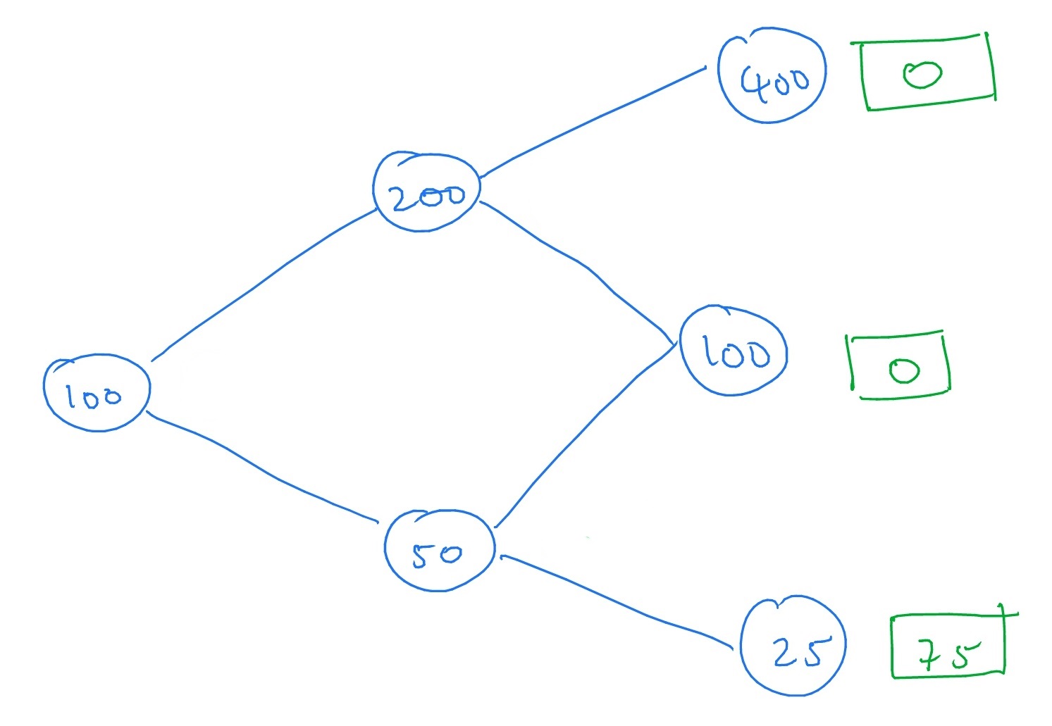
By (5.3), the risk free probabilities in this case are
\[q_u=\frac {(1+0.25)-0.5}{2.0-0.5}=0.5,\quad q_d=1-q_u=0.5.\]
Using Proposition 5.2.6 recursively, as in Section 5.6, we can put in the value of the European put option at all nodes back to time \(0\), giving
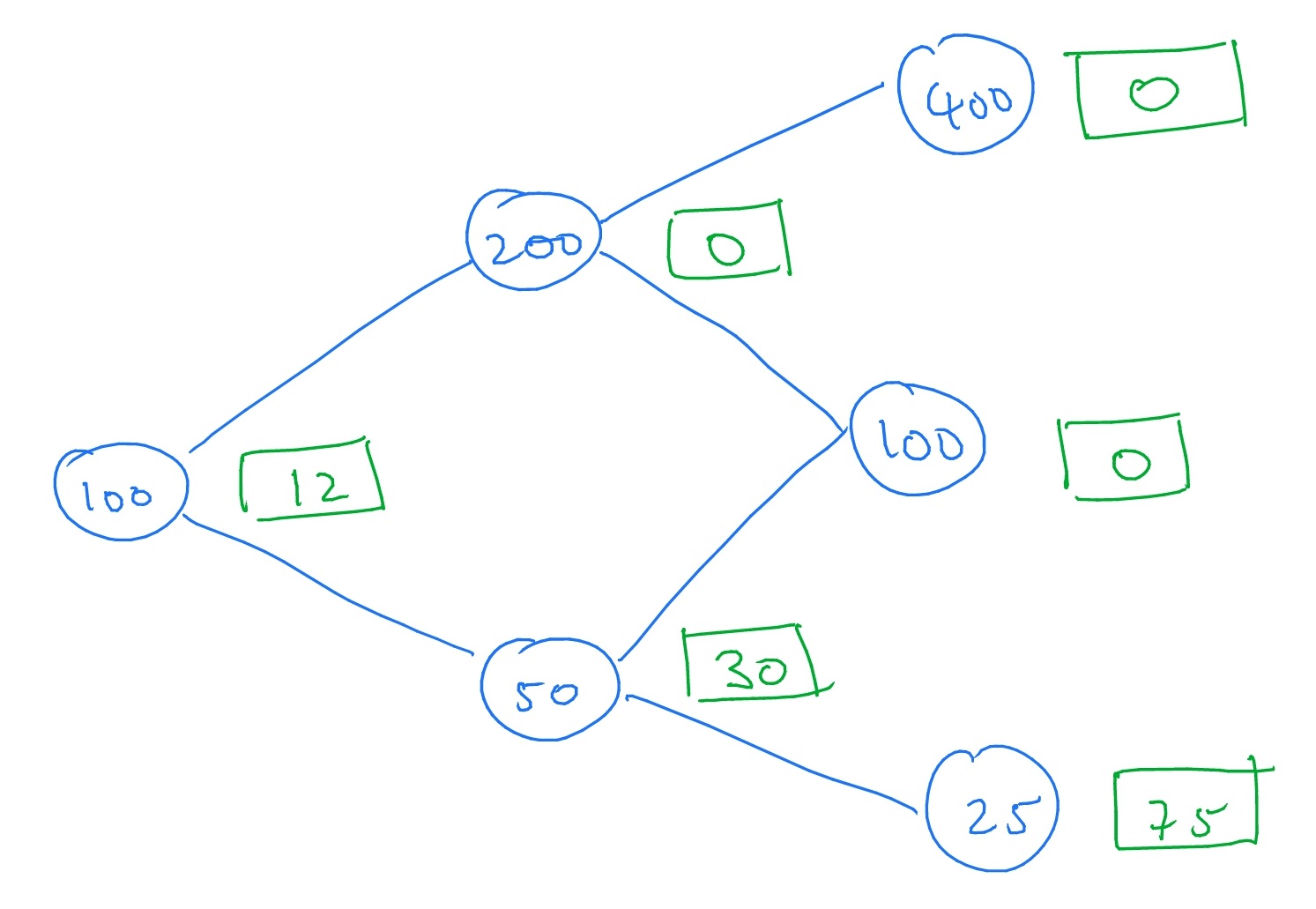
Hence, the value of our European put option at time \(0\) is \(12\).
Changing the values of \(p_u\) and \(p_d\) do not alter value of our put option, since \(p_u\) and \(p_d\) do not appear in the pricing formulae.
-
5.7 A tree-like diagram of the possible changes in stock price, with the value of the option at all nodes of the tree shown in (green) square boxes, and hedging portfolios \(h=(x,y)\) written (in red) for each node of the tree:
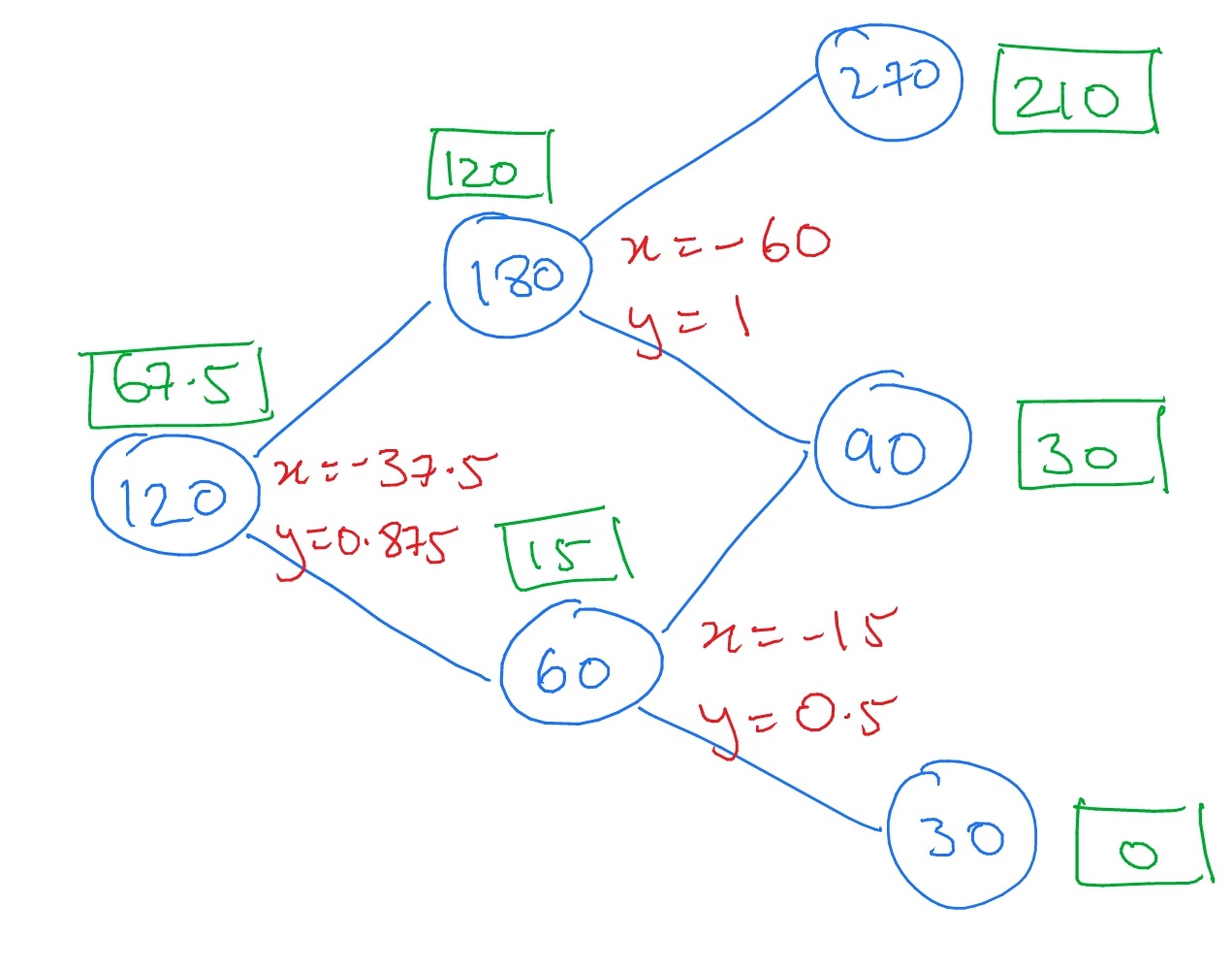
The hedging portfolios are found by solving linear equations of the form \(x+dSy=\wt {\Phi }(dS)\), \(x+uSy=\wt {\Phi }(uD)\), where \(\wt \Phi \) is the contingent claim and \(S\) the initial stock price of the one period model associated to the given node. The value of the contingent claim at each node is then inferred from the hedging portfolio as \(V=x+Sy\).
-
5.8 A tree-like diagram of the possible changes in stock price, with the value of the option at all nodes of the tree shown in (green) square boxes, and hedging portfolios \(h=(x,y)\) written (in red) for each node of the tree:
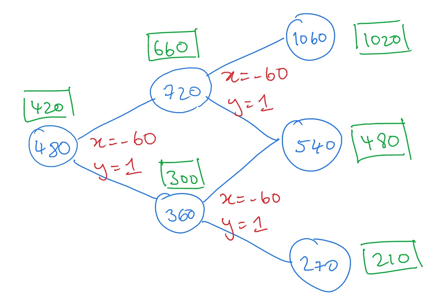
The hedging portfolios are found by solving linear equations of the form \(x+dSy=\wt {\Phi }(dS)\), \(x+uSy=\wt {\Phi }(uD)\), where \(\wt \Phi \) is the contingent claim and \(S\) the initial stock price of the one period model associated to the given node. The value of the contingent claim at each node is then inferred from the hedging portfolio as \(V=x+Sy\).
The hedging portfolio is the same at each node. This is because the contingent claim of our call option always exceeds zero i.e. we are certain that at time \(T=2\) we would want to exercise our call option and buy a single unit of stock for a price \(K=60\). Since there is no interest payable on cash, this means that we can replicate our option (at all times) by holding a single unit of stock, and \(-60\) in cash.
-
5.9 We have that \((S_t)\) is adapted (see Section 5.4) and since \(S_t\in (d^t,u^t)\) we have also that \(S_t\in L^1\). Hence, \(S_t\) is a martingale under \(\P \) if and only if \(\E ^\P [S_{t+1}\|\F _t]=S_t\). That is if
\(\seteqnumber{0}{A.}{4}\)\begin{align*} \E ^\P [S_{t+1}\|\F _t]&=\E [Z_{t+1}S_{t}\|\mc {F}_t]\\ &=S_t\E ^\P [Z\|\mc {F}_t]\\ &=S_t\E ^\P [Z] \end{align*} is equal to \(S_t\). Hence, \(S_t\) is a martingale under \(\P \) if and only if \(\E ^\P [Z_{t+1}]=up_u+dp_d=1.\)
Now consider \(M_t=\log S_t\), and assume that \(0<d<u\) and \(0<s\), which implies \(S_t>0\). Since \(S_t\) is adapted, so is \(M_t\). Since \(S_t\in S_t\in (d^t,u^t)\) we have \(M_t\in (t \log d, t\log u)\) so also \(M_t\in L^1\). We have
\[M_t=\log \l (S_0\prod \limits _{i=1}^tZ_i\r )=\log (S_0)+\sum \limits _{i=1}^t Z_i.\]
Hence,
\(\seteqnumber{0}{A.}{4}\)\begin{align*} \E ^\P [M_{t+1}|\mc {F}_t]&=\log S_0+\sum \limits _{i=1}^{t}\log (Z_i)+\E [\log (Z_{t+1})\|\mc {F}_t]\\ &=M_t+\E ^\P [\log Z_{t+1}]\\ &=M_t+p_u\log u + p_d\log d. \end{align*} Here we use taking out what is known, since \(S_0\) and \(Z_i\in m\mc {F}_t\) for \(i\leq t\), and also that \(Z_{t+1}\) is independent of \(\mc {F}_t\). Hence, \(M_t\) is a martingale under \(\P \) if and only if \(p_u\log u + p_d\log d=0\).
Chapter 6
-
6.1 Since \(X_n\geq 0\) we have
\[\E [|X_n-0|]=\E [X_n]=\tfrac 122^{-n}=2^{-(n+1)}\]
which tends to \(0\) as \(n\to \infty \). Hence \(X_n\to 0\) in \(L^1\). Lemma 6.1.2 then implies that also \(X_n\to 0\) in probability and in distribution. Also, \(0\leq X_n\leq 2^{-n}\) and \(2^{-n}\to 0\), so by the sandwich rule we have \(X_n\to 0\) as \(n\to \infty \), and hence \(\P [X_n\to 0]=1\), which means that \(X_n\to 0\) almost surely.
-
-
(a) We have \(X_n\stackrel {L^1}{\to } X\) and hence
\[\l |\E [X_n]-\E [X]\r |=|\E [X_n-X]|\leq \E [|X_n-X|]\to 0.\]
Here we use the linearity and absolute value properties of expectation. Hence, \(\E [X_n]\to \E [X]\).
-
(b) Let \(X_1\) be a random variable such that \(\P [X_1=1]=\P [X_1=-1]=\frac 12\) and note that \(\E [X_1]=0\). Set \(X_n=X_1\) for all \(n\geq 2\), which implies that \(\E [X_n]=0\to 0\) as \(n\to \infty \). But \(\E [|X_n-0|]=\E [|X_n|]=1\) so \(X_n\) does not converge to \(0\) in \(L^1\).
-
-
6.3 We have \(X_n=X\) when \(U=2\), and \(|X_n-X|=\frac {1}{n}\) when \(U=0,1\). Hence, \(|X_n-X|\leq \frac {1}{n}\) and by monotonicity of \(\E \) we have
\[\E \l [|X_n-X|\r ]\leq \frac {1}{n}\to 0\quad \text { as }n\to \infty ,\]
which means that \(X_n\stackrel {L^1}{\to }X\).
We can write
\(\seteqnumber{0}{A.}{4}\)\begin{align*} \P [X_n\to X] &=\P [X_n\to X, U=0]+\P [X_n\to X, U=1] + \P [X_n\to X, U=2]\\ &=\P [1+\frac {1}{n}\to 1, U=0]+\P [1-\frac {1}{n}\to 1, U=1] + \P [0\to 0, U=2]\\ &=\P [U=0]+\P [U=1]+\P [U=2]\\ &=1. \end{align*} Hence, \(X_n\stackrel {a.s.}{\to } X\).
By Lemma 6.1.2, it follows that also \(X_n\to X\) in probability and in distribution.
-
6.4 We have \(X_n=X_1=1-Y\) for all \(n\), so \(Y=0\iff X_n=1\) and \(Y=1\iff X_n=0\). Hence \(|Y-X_n|=1\) for all \(n\). So, for example, with \(a=\frac 12\) we have \(\P [|X_n-Y|\geq a]=1\), which does not tend to zero as \(n\to \infty \). Hence \(X_n\) does not converge to \(Y\) in probability.
However, \(X_n\) and \(y\) have the same distribution, given by
\[\P [Y\leq x]=\P [X_n\leq x]= \begin {cases} 0 & \text { if } x<0\\ \frac 12 & \text { if } x\in [0,1)\\ 1 & \text { if }x\geq 1 \end {cases} \]
so we do have \(\P [X_n\leq x]\to \P [Y\leq x]\) as \(n\to \infty \). Hence \(X_n\stackrel {d}{\to }Y\).
-
6.5 Let \((X_n)\) be the sequence of random variables from 6.1. Define \(Y_n=X_1+X_2+\ldots +X_n\).
-
(a) For each \(\omega \in \Omega \), we have \(Y_{n+1}(\omega )=Y_n(\omega )+X_{n+1}(\omega )\). Hence, \((Y_n(\omega )\) is an increasing sequence. Since \(X_n(\omega )\leq 2^{-n}\) for all \(n\) we have
\[|Y_n(\omega )|\leq 2^{-1}+2^{-2}+\ldots +2^{-n}\leq \sum \limits _{i=1}^\infty 2^{-i}=1,\]
meaning that the sequence \(Y_n(\omega )\) is bounded above by \(1\).
-
(b) Hence, since bounded increasing sequences converge, for any \(\omega \in \Omega \) the sequence \(Y_n(\omega )\) converges.
-
(c) The value of \(Y_1\) is either \(0\) or \(\frac 12\), both with probability \(\frac 12\). The value of \(Y_2\) is either \(0,\frac 14,\frac 12,\frac 34\), all with probability \(\frac 14\). The value of \(Y_3\) is either \(0,\frac 18,\frac 14,\frac 38,\frac 12,\frac 58,\frac 34,\frac 78\) all with probability \(\frac 18\).
-
(d) We can guess from (c) that the \(Y_n\) are becoming more and more evenly spread across \([0,1]\), so we expect them to approach a uniform distribution as \(n\to \infty \).
-
(e) We will use induction on \(n\). Our inductive hypothesis is
-
(IH)\(_n\): For all \(k=0,1,\ldots ,2^n-1\), it holds that \(\P [Y_n=k2^{-n}]=2^{-n}\).
In words, this says that \(Y_n\) is uniformly distributed on \(\{k2^{-n}\-k=0,1,\ldots ,2^n-1\}\).
For the case \(n=1\), we have \(Y_1=X_1\) so \(\P [Y_1=0]=\P [Y_1=\tfrac 12]=\tfrac 12\), hence (IH)\(_1\) holds.
Now, assume that (IH)\(_n\) holds. We want to calculate \(\P [Y_{n+1}=k2^{-(n+1)}\) for \(k=0,1,\ldots ,2^{n+1}-1\). We consider two cases, dependent on whether \(k\) is even or odd.
-
• If \(k\) is even then we can write \(k=2j\) for some \(j=0,\ldots ,2^n-1\). Hence,
\(\seteqnumber{0}{A.}{4}\)\begin{align*} \P [Y_{n+1}=k2^{-(n+1)}] &=\P [Y_{n+1}=j2^{-n}]\\ &=\P [Y_n=j2^{-n}\text { and }X_{n+1}=0]\\ &=\P [Y_n=j2^{-n}]\P [X_{n+1}=0]\\ &=2^{-n}\tfrac 12\\ &=2^{-(n+1)}. \end{align*} Here we use that \(Y_n\) and \(X_{n+1}\) are independent, and use (IH)\(_n\) to calculate \(\P [Y_n=j2^{-n}]\).
-
• Alternatively, if \(k\) is odd then we can write \(k=2j+1\) for some \(j=0,\ldots ,2^n-1\). Hence,
\(\seteqnumber{0}{A.}{4}\)\begin{align*} \P [Y_{n+1}=k2^{-(n+1)}] &=\P [Y_{n+1}=j2^{-n}+2^{-(n+1)}]\\ &=\P [Y_n=j2^{-n}\text { and }X_{n+1}=2^{-(n+1)}]\\ &=\P [Y_n=j2^{-n}]\P [X_{n+1}=2^{-(n+1)}]\\ &=2^{-n}\tfrac 12\\ &=2^{-(n+1)}. \end{align*} Here, again, we use that \(Y_n\) and \(X_{n+1}\) are independent, and use (IH)\(_n\) to calculate \(\P [Y_n=j2^{-n}]\).
In both cases we have shown that \(\P [Y_{n+1}=k2^{-(n+1)}]=2^{-(n+1)}\), hence (IH)\(_{n+1}\) holds.
-
-
(f) We know that \(Y_n\to Y\) almost surely, hence by Lemma 6.1.2 the convergence also holds in distribution. Hence \(\P [Y_n\leq a]\to \P [Y\leq a]\).
From part (e), for any \(a\in [0,1]\) we have
\[(k-1)2^{-n}\leq a<k2^{-n}\quad \ra \quad \P [Y_n\leq a]=k2^{-n}.\]
Hence \(a\leq \P [Y_n\leq a]\leq a+2^{-n}\), and the sandwich rule tells us that \(\P [Y_n\leq a]\to a\). Hence \(\P [Y\leq a]=a\), for all \(a\in [0,1]\), which means that \(Y\) has a uniform distribution on \([0,1]\).
-
-
6.7 Since \(\1\{X\leq n+1\}\geq 1\{X\leq n\}\) we have \(X_{n+1}\geq X_n\), and since \(X>0\) we have \(X_n\geq 0\). Further, for all \(\omega \in \Omega \), whenever \(X(w)<n\) we have \(X_n(\omega )=X(\omega )\), and since \(\P [X(\omega )<\infty ]=1\) this means that \(\P \l [X_n(\omega )\to X(\omega )\r ]=1\). Hence \(X_n\stackrel {a.s.}{\to } X\).
Therefore, the monotone convergence theorem applies and \(\E [X_n]\to \E [X]\).
-
6.6 Define \(X_n=-Y_n\). Then \(X_n\geq 0\) and \(X_{n+1}\geq X_n\), almost surely. Hence, \((X_n)\) satisfies the conditions for the dominated convergence theorem and there exists a random variable \(X\) such that \(X_n\stackrel {a.s.}{\to }X\) and \(\E [X_n]\to \E [X]\). Define \(Y=-X\) and then we have \(Y_n\stackrel {a.s.}{\to }Y\) and \(\E [Y_n]\to \E [Y]\).
-
-
(a) The equation
\(\seteqnumber{0}{A.}{4}\)\begin{equation} \label {eq:fubini_mct_pre} \E \l [\sum _{i=1}^n X_i\r ]=\sum _{i=1}^n \E [X_i] \end{equation}
follows by iterating the linearity property of \(\E \) \(n\) times (or by a trivial induction). However, in \(\E \big [\sum _{i=1}^\infty X_i\big ]=\sum _{i=1}^\infty \E [X_i]\) both sides are defined by infinite sums, which are limits, and the linearity property does not tell us anything about limits.
-
(b) We’ll take a limit as \(n\to \infty \) on each side of (A.5). We’ll have to justify ourselves in each case.
First, consider the right hand side. Since we have \(X_n\geq 0\) almost surely, \(\E [X_n]\geq 0\) by monotonicity of \(\E \). Therefore, \(\sum _{i=1}^n \E [X_i]\) is an increasing sequence of real numbers. Hence it is convergent (either to a real number or to \(+\infty \)) and, by definition of an infinite series, the limit is written \(\sum _{i=1}^\infty \E [X_i]\).
Now, the left hand side, and here we’ll need the monotone convergence theorem. Define \(Y_n=\sum _{i=1}^n X_i\). Then \(Y_{n+1}-Y_n=X_{n+1}\geq 0\) almost surely, so \(Y_{n+1}\geq Y_n\). Since \(X_i\geq 0\) for all \(i\), also \(Y_n\geq 0\), almost surely. Hence the monotone convergence theorem applies and \(\E [Y_n]\to \E [Y_\infty ]\) where \(Y_\infty =\sum _{i=1}^\infty X_i\).
Putting both sides together (and using the uniqueness of limits to tell us that the limits on both sides must be equal as \(n\to \infty \)) we obtain that \(\E \big [\sum _{i=1}^\infty X_i\big ]=\sum _{i=1}^\infty \E [X_i]\).
-
(c) Since \(\P [X_i=1]=\P [X_i=-1]\), we have \(\E [X_i]=0\) and hence also \(\sum _{i=1}^\infty \E [X_i]=0\). However, the limit \(\sum _{i=1}^\infty X_i\) is not well defined, because \(Y_n=\sum _{i=1}^n X_i\) oscillates (it jumps up/down by \(\pm 1\) on each step) and does not converge. Hence, in this case \(\E \big [\sum _{i=1}^\infty X_i\big ]\) is not well defined.
-
-
-
(a) We have both \(\P [X_n\leq x]\to \P [X\leq x]\) and \(\P [X_n\leq x]\to \P [Y\leq x]\), so by uniqueness of limits for real sequences, we have \(\P [X\leq x]=\P [Y\leq x]\) for all \(x\in \R \). Hence, \(X\) and \(Y\) have the same distribution (i.e. they have the same distribution functions \(F_X(x)=F_Y(x)\)).
-
(b) By definition of convergence in probability, for any \(a>0\), for any \(\epsilon >0\) there exists \(N\in \N \) such that, for all \(n\geq N\),
\[\P [|X_n-X|>a]<\epsilon \hspace {1pc}\text { and }\hspace {1pc}\P [|X_n-Y|>a]<\epsilon .\]
By the triangle inequality we have
\(\seteqnumber{0}{A.}{5}\)\begin{equation} \label {eq:ps_uniq_limit} \P [|X-Y|>2a]=\P [|X-X_n+X_n-Y|>2a]\leq \P [|X-X_n|+|X_n-Y|>2a]. \end{equation}
If \(|X-X_n|+|X_n-Y|>2a\) then \(|X-X_n|>a\) or \(|X_n-Y|>a\) (or possibly both). Hence, continuing (A.6),
\[\P [|X-Y|>2a]\leq \P [|X_n-X|>a]+\P [|X_n-Y|>a]\leq 2\epsilon .\]
Since this is true for any \(\epsilon >0\) and any \(a>0\), we have \(\P [X=Y]=1\).
-
-
6.7 Suppose (aiming for a contradiction) that there exists and random variable \(X\) such that \(X_n\to X\) in probability. By the triangle inequality we have
\[|X_n-X_{n+1}|\leq |X_n-X|+|X-X_{n+1}|\]
Hence, if \(|X_n-X_{n+1}|>1\) then \(|X_n-X|>\frac 12\) or \(|X_{n+1}-X|>\frac 12\) (or both). Therefore,
\[\P \l [|X_n-X_{n+1}|>1\r ]\leq \P \l [|X_n-X|>\tfrac 12\r ]+\P \l [|X_{n+1}-X|>\tfrac 12\r ].\]
Since \(X_n\to X\) in probability, the right hand side of the above tends to zero as \(n\to \infty \). This implies that
\[\P \l [|X_n-X_{n+1}|>1\r ]\to 0\]
as \(n\to \infty \). But, \(X_n\) and \(X_{n+1}\) are independent and \(\P [X_n=1,X_{n+1}=0]=\frac 14\) so \(\P [|X_n-X_{n+1}|>1]\geq \frac 14\) for all \(n\). Therefore we have a contradiction, so there is no \(X\) such that \(X_n\to X\) in probability.
Hence, by Lemma 6.1.2, we can’t have any \(X\) such that \(X_n\to X\) almost surely or in \(L^1\) (since it would imply convergence in probability).
Chapter 7
-
-
(a) We have \((C\circ M)_n=\sum _{i=1}^n 0(S_i-S_{i-1})=0.\)
-
(b) We have \((C\circ M)_n=\sum _{i=1}^n 1(S_i-S_{i-1})=S_n-S_0=S_n.\)
-
(c) We have
\(\seteqnumber{0}{A.}{6}\)\begin{align*} (C\circ M)_n &=\sum _{i=1}^n S_{i-1}(S_i-S_{i-1})\\ &=\sum _{i=1}^n (X_1+\ldots +X_{i-1})X_i\\ &=\frac 12\l (\sum _{i=1}^n X_i\r )^2-\frac 12\sum _{i=1}^n X_i^2\\ &=\frac {S_n^2}{2}-\frac {n}{2} \end{align*} In the last line we use that \(X_i^2=1\).
-
-
7.2 We have
\(\seteqnumber{0}{A.}{6}\)\begin{align*} (X\circ M)_n &=\sum \limits _{i=1}^n (\alpha C_{n-1}+\beta D_{n-1})(M_n-M_{n-1})\\ &=\alpha \sum \limits _{i=1}^n C_{n-1}(M_n-M_{n-1}) + \beta \sum \limits _{i=1}^n D_{n-1}(M_n-M_{n-1})\\ &=\alpha (C\circ M)_n + \beta (C\circ M)_n \end{align*} as required.
-
-
(a) We note that
\[|S_n|\leq \sum \limits _{i=1}^n|X_i|\leq \sum \limits _{i=1}^n 1=n<\infty .\]
Hence \(S_n\in L^1\). Since \(X_i\in \mc {F}_n\) for all \(i\leq n\), we have also that \(S_n\in m\mc {F}_n\). Lastly,
\(\seteqnumber{0}{A.}{6}\)\begin{align*} \E [S_{n+1}\|\mc {F}_n] &=\E [S_n+X_{n+1}\|\mc {F}_n]\\ &=S_n+\E [X_{n+1}]\\ &=S_n. \end{align*} Therefore, \(S_n\) is a martingale. In the above, in the second line we use that \(S_n\in m\mc {F}_n\) and that \(X_{n+1}\) is independent of \(\mc {F}_n\). To deduce the last line we use that \(\E [X_i]=\frac {1}{2n^2}(1)=\frac {1}{2n^2}(-1)+(1-\frac {1}{n^2})(0)=0\).
We next check that \(S_n\) is uniformly bounded in \(L^1\). We have \(\E [|X_i|]=\frac {1}{2i^2}|1|+\frac {1}{2i^2}|-1|+(1-\frac {1}{i^2})|0|=\frac {1}{i^2}\). Using that \(|S_n|\leq |X_1|+\ldots +|X_n|\), monotonicity of expectations gives that
\[\E [|S_n|]\leq \sum _{i=1}^n \E [|X_i|]\leq \sum _{i=1}^n \frac {1}{i^2}\leq \sum _{i=1}^\infty \frac {1}{i^2}<\infty .\]
Hence \(\sup _n\E [|S_n|]<\infty \), so \((S_n)\) is uniformly bounded in \(L^1\).
Therefore, the martingale convergence theorem applies, which gives that there exists some real-valued random variable \(S_\infty \) such that \(S_n\stackrel {a.s.}{\to }S_\infty \).
-
(b) Note that \((S_n)\) takes values in \(\Z \) and that, from part (b), almost surely we have that \(S_n\) converges to a real value. It follows immediately by Lemma 7.4.1 that (almost surely) there exists \(N\in \N \) such that \(S_n=S_\infty \) for all \(n\geq N\).
-
-
7.4 Here’s some R code to plot \(1000\) time-steps of the symmetric random walk. Changing the value given to set.seed will generate a new sample.
> T=1000
> set.seed(1)
> x=c(0,2*rbinom(T-1,1,0.5)-1)
> y=cumsum(x)
> par(mar=rep(2,4))
> plot(y,type="l")
Adapting it to plot the asymmetric case and the random walk from exercise 7.3 is left for you.
In case you prefer Python, here’s some Python code that does the same job. (I prefer Python.)
import numpy as np
import matplotlib.pyplot as plt

p = 0.5
rr = np.random.random(1000)
step = 2*(rr < p) - 1

start = 0
positions = [start]
for x in step:
    positions.append(positions[-1] + x)

plt.plot(positions)
plt.show()
Extending this code as suggested is left for you. For the last part, the difference in behaviour that you should notice from the graph is that the walk from Exercise 7.3 eventually stops moving (at some random time), whereas the random walk from Q2 of Assignment 3 never keeps moving but makes smaller and smaller steps.
-
7.5 We will argue by contradiction. Suppose that \((M_n)\) was uniformly bounded in \(L^1\). Then the martingale convergence theorem would give that \(M_n\stackrel {a.s.}{\to }M_\infty \) for some real valued random variable \(M_\infty \). However, \(M_n\) takes values in \(\Z \) and we have \(M_{n+1}\neq M_n\) for all \(n\), so Lemma 7.4.1 gives that \((M_n)\) cannot converge almost surely. This is a contradiction.
-
-
(a) Take the offspring distribution to be \(\P [G=0]=1\). Then \(Z_1=0\), and hence \(Z_n=0\) for all \(n\geq 1\), so \(Z_n\) dies out.
-
(b) Take the offspring distribution to be \(\P [G=2]=1\). Then \(Z_{n+1}=2Z_n\), so \(Z_n=2^n\), and hence \(Z_n\to \infty \).
-
-
-
(a) We have
\(\seteqnumber{0}{A.}{6}\)\begin{align*} \E [M_{n+1}\|\mc {F}_n] &=\E \l [M_{n+1}\1\{n^{th}\text { draw is red}\}\,\Big |\,\mc {F}_n\r ] +\E \l [M_{n+1}\1\{n^{th}\text { draw is black}\}\,\Big |\,\mc {F}_n\r ]\\ &=\E \l [\frac {B_n}{n+3}\,\1\{n^{th}\text { draw is red}\}\,\Big |\,\mc {F}_n\r ] +\E \l [\frac {B_n+1}{n+3}\,\1\{n^{th}\text { draw is black}\}\,\Big |\,\mc {F}_n\r ]\\ &=\frac {B_n}{n+3}\E \l [\1\{n^{th}\text { draw is red}\}\,\Big |\,\mc {F}_n\r ] +\frac {B_n+1}{n+3}\E \l [\,\1\{n^{th}\text { draw is black}\}\,\Big |\,\mc {F}_n\r ]\\ &=\frac {B_n}{n+3}\frac {B_n}{n+2}+\frac {B_n+1}{n+3}\l (1-\frac {B_n}{n+2}\r )\\ &=\frac {B_n^2}{(n+2)(n+3)}+\frac {B_n(n+2)+(n+2)-B_n^2-B_n}{(n+2)(n+3)}\\ &=\frac {(n+1)B_n+(n+2)}{(n+2)(n+3)} \end{align*} This is clearly not equal to \(M_n=\frac {B_n}{n+2}\), so \(M_n\) is not a martingale.
This result might be rather surprising, but we should note that the urn process here is not ‘fair’, when considered in terms of the proportion of (say) red balls. If we started with more red balls than black balls, then over time we would expect to see the proportion of red balls reduce towards \(\frac 12\), as we see in part (b):
-
(b) Your conjecture should be that, regardless of the initial state of the urn, \(\P [M_n\to \frac 12\text { as }n\to \infty ]=1\). (It is true.)
-
-
-
(a) Let \(B_n\) be the number of red balls in the urn at time \(n\), and then \(M_n=\frac {B_n}{K}\). Let us abuse notation slightly and write \(B=r\) for the event that the ball \(X\) is red, and \(X=b\) for the event that the ball \(X\) is black. Let \(X_1\) denote the first ball drawn on the \((n+1)^{th}\) draw, and \(X_2\) denote the second ball drawn.
Let \(\mc {F}_n=\sigma (B_1,\ldots ,B_n)\). It is clear that \(M_n\in [0,1]\), so \(M_n\in L^1\), and that \(M_n\) is measurable with respect to \(\mc {F}_n\). We have
\(\seteqnumber{0}{A.}{6}\)\begin{align*} \E [M_{n+1}\|\mc {F}_{n}] &=\E \l [M_{n+1}\1_{\{X_1=r, X_2=r\}}\|\mc {F}_n\r ]+\E \l [M_{n+1}\1_{\{X_1=r, X_2=b\}}\|\mc {F}_n\r ]\\ &\hspace {2pc}+\E \l [M_{n+1}\1_{\{X_1=b, X_2=r\}}\|\mc {F}_n\r ]+\E \l [M_{n+1}\1_{\{X_1=b, X_2=b\}}\|\mc {F}_n\r ]\\ &=\E \l [\frac {B_n}{K}\1_{\{X_1=r, X_2=r\}}\|\mc {F}_n\r ]+\E \l [\frac {B_n+1}{K}\1_{\{X_1=r, X_2=b\}}\|\mc {F}_n\r ]\\ &\hspace {2pc}+\E \l [\frac {B_n-1}{K}\1_{\{X_1=b, X_2=r\}}\|\mc {F}_n\r ]+\E \l [\frac {B_n}{K}\1_{\{X_1=b, X_2=b\}}\|\mc {F}_n\r ]\\ &=\frac {B_n}{K}\E \l [\1_{\{X_1=r, X_2=r\}}\|\mc {F}_n\r ]+\frac {B_n+1}{K}\E \l [\1_{\{X_1=r, X_2=b\}}\|\mc {F}_n\r ]\\ &\hspace {2pc}+\frac {B_n-1}{K}\E \l [\1_{\{X_1=b, X_2=r\}}\|\mc {F}_n\r ]+\frac {B_n}{K}\E \l [\1_{\{X_1=b, X_2=b\}}\|\mc {F}_n\r ]\\ &=\frac {B_n}{K}\frac {B_n}{K}\frac {B_n}{K}+\frac {B_n+1}{K}\frac {B_n}{K}\frac {K-B_n}{K}\\ &\hspace {2pc}+\frac {B_n-1}{K}\frac {K-B_n}{K}\frac {B_n}{K}+\frac {B_n}{K}\frac {K-B_n}{K}\frac {K-B_n}{K}\\ &=\frac {1}{K^3}\l (B_n^3+2B_n^2(K-B_n)+B_n(K-B)n-B_n(K-B_n)+B_n(K-B_n)^2\r )\\ &=\frac {1}{K^3}\l (K^2B_n\r )\\ &=M_n \end{align*}
-
(b) Since \(M_n\in [0,1]\) we have \(\E [|M_n|]\leq 1\), hence \(M_n\) is uniformly bounded in \(L^1\). Hence, by the martingale convergence theorem there exists a random variable \(M_\infty \) such that \(M_n\stackrel {a.s.}{\to }M_\infty \).
Since \(M_n=\frac {B_n}{K}\), this means that also \(B_n\stackrel {a.s.}{\to }KM_\infty \). However, \(B_n\) is integer valued so, by Lemma 7.4.1, if \(B_n\) is to converge then it must eventually become constant. This can only occur if, eventually, the urn contains either (i) only red balls or (ii) only black balls.
In case (i) we have \(M_n=0\) eventually, which means that \(M_\infty =0\). In case (ii) we have \(M_n=1\) eventually, which means that \(M_\infty =1\). Hence, \(M_\infty \in \{0,1\}\) almost surely.
-
-
-
(a) Consider the usual Pólya urn, from Section 4.2, started with just one red ball and one black ball. After the first draw is complete we have two possibilities:
-
1. The urn contains one red ball and two black balls.
-
2. The urn contains two red balls and one black ball.
In the first case we reach precisely the initial state of the urn described in 7.9. In the second case we also reach the initial state of the urn described in 7.9, but with the colours red and black swapped.
If \(M_n\stackrel {a.s.}{\to } 0\), then in the first case the fraction of red balls would tend to zero, and (by symmetry of colours) in the second case the limiting fraction of black balls would tend to zero; thus the limiting fraction of black balls would always be either \(1\) (the first case) or \(0\) (the second case). However, we know from Proposition 7.4.3 that the limiting fraction of black balls is actually uniform on \((0,1)\). Hence, \(\P [M_n\to 0]=0\).
-
-
(b) You should discover that having a higher proportion of initial red balls makes it more likely for \(M_\infty \) (the limiting proportion of red balls) to be closer to \(1\). However, since \(M_\infty \) is a random variable in this case, you may need to take several samples of the process (for each initial condition that you try) to see the effect.
Follow-up challenge question: In fact, the limiting value \(M_\infty \) has a Beta distribution, \(Be(\alpha ,\beta )\). You may need to look up what this means, if you haven’t seen the Beta distribution before. Consider starting the urn with \(n_1\) red and \(n_2\) black balls, and see if you can use your simulations to guess a formula for \(\alpha \) and \(\beta \) in terms of \(n_1\) and \(n_2\) (the answer is a simple formula!).
-
-
-
(a) We have that \((M_n)\) is a non-negative martingale, hence \(\sup _n\E [|M_n|]=\sup _n\E [M_n]=\E [M_0]=1\). Thus \((M_n)\) is uniformly bounded in \(L^1\) and the (first) martingale convergence theorem applies, giving that \(M_n\stackrel {a.s.}{\to }M_\infty \) for a real valued \(M_\infty \). Since \(M_n\geq 0\) almost surely we must have \(M_\infty \geq 0\) almost surely.
-
(b) The possible values of \(M_n\) are \(W=\{(q/p)^{z}\-z\in \Z \}\). Note that \(M_{n+1}\neq M_n\) for all \(n\in \N \).
On the event that \(M_\infty >0\) there exists \(\epsilon >0\) such that \(M_n\geq \epsilon \) for all sufficiently large \(n\). Choose \(m\in \N \) such that \((q/p)^m\leq \epsilon \) and then for all sufficiently large \(n\) we have \(M_n\in W_m=\{(q/p)^z\-z\geq m, z\in \Z \}\). For such \(n\), since \(M_n\neq M_{n+1}\) we have \(|M_n-M_{n+1}|\geq |(q/p)^m-(q/p)^{m-1}|>0\), which implies that \((M_n)\) could not converge. Hence, the only possible almost sure limit is \(M_\infty =0\).
If \((M_n)\) was uniformly bounded in \(L^2\) then by the (second) martingale convergence theorem we would have \(\E [M_n]\to \E [M_\infty ]\). However \(\E [M_n]=\E [M_0]=1\) and \(\E [M_\infty ]=0\), so this is a contradiction. Hence \((M_n)\) is not uniformly bounded in \(L^2\).
-
(c) We have \((q/p)^S_n\stackrel {a.s.}{\to }0\). Noting that \(q/p>1\) and hence \(\log (q/p)>0\), taking logs gives that \(S_n\log (q/p)\stackrel {a.s.}{\to }-\infty \), which gives \(S_n\stackrel {a.s.}{\to }-\infty \).
For the final part, if \((S_n)\) is a simple asymmetric random walk with upwards drift, then \((-S_n)\) is a simple asymmetric random walk with downwards drift. Applying what we’ve just discovered thus gives \(-S_n\stackrel {a.s.}{\to }-\infty \), and multiplying by \(-1\) gives the required result.
-
-
-
(a) This is a trivial induction: if \(S_n\) is even then \(S_{n+1}\) is odd, and vice versa.
-
(b) By part (a), \(p_{2n+1}=0\) since \(0\) is an even number and \(S_{2n+1}\) is an odd number.
If \(S_n\) is to start at zero and reach zero at time \(2n\), then during time \(1,2,\ldots ,2n\) it must have made precisely \(n\) steps upwards and precisely \(n\) steps downwards. The number of different ways in which the walk can do this is \(\binom {2n}{n}\) (we are choosing exactly \(n\) steps on which to go upwards, out of \(2n\) total steps). Each one of these ways has probability \((\frac 12)^{2n}\) of occurring, so we obtain \(p_{2n}=\binom {2n}{n}2^{-2n}\).
-
(c) From (b) we note that
\[p_{2(n+1)}=\frac {(2n+2)(2n+1)}{(n+1)(n+1)}2^{-2}p_{2n}=2\l (\frac {2n+1}{n+1}\r )2^{-2}p_n=\l (\frac {2n+1}{2n+2}\r )p_{2n}=\l (1-\frac {1}{2(n+1)}\r )\frac 12 p_{2n}.\]
Hence, using the hint, we have
\[p_{2(n+1)}\leq \exp \l (-\frac {1}{2(n+1)}\r )p_{2n}.\]
Iterating this formula obtains that
\(\seteqnumber{0}{A.}{6}\)\begin{align} p_{2n} &\leq \exp \l (-\frac {1}{2n}\r )\exp \l (-\frac {1}{2(n-1)}\r )\ldots \exp \l (-\frac {1}{2(1)}\r )p_0\notag \\ &=\exp \l (-\frac {1}{2}\sum \limits _{i=1}^n\frac {1}{i}\r ).\label {eq:ssrw_p2n} \end{align} Recall that \(\sum _{i=1}^n\frac {1}{i}\to \infty \) as \(n\to \infty \), and that \(e^{-x}\to 0\) as \(x\to \infty \). Hence, the right hand side of the expression above tends to zero as \(n\to \infty \). Hence, since \(p_{n}\geq 0\), by the sandwich we have \(p_{2n}\to 0\) as \(n\to \infty \).
-
-
-
(a) We note that
\(\seteqnumber{0}{A.}{7}\)\begin{align*} \E \l [\frac {S_{n+1}}{f(n+1)}\,\Big |\,\mc {F}_n\r ]&=\frac {S_n}{f(n+1)}+\frac {1}{f(n+1)}\E [X_{n+1}\|\mc {F}_n]\notag \\ &=\frac {S_n}{f(n+1)}+\frac {1}{f(n+1)}\E [X_{n+1}]\notag \\ &=\frac {S_n}{f(n+1)} \end{align*} Here we use that \(S_n\in m\mc {F}_n\) and that \(X_{n+1}\) is independent of \(\mc {F}_n\).
Since \(\frac {S_n}{f(n)}\) is a martingale we must have
\(\seteqnumber{0}{A.}{7}\)\begin{equation} \label {eq:ESnfn} \frac {S_n}{f(n+1)}=\frac {S_n}{f(n)}. \end{equation}
Since \(\P [S_n\neq 0]>0\) this implies that \(\frac {1}{f(n+1)}=\frac {1}{f(n)}\), which implies that \(f(n+1)=f(n)\). Since this holds for any \(n\), we have \(f(1)=f(n)\) for all \(n\); so \(f\) is constant.
-
(b) If \(\frac {S_n}{f(n)}\) is to be a supermartingale then, in place of (A.8), we would need
\(\seteqnumber{0}{A.}{8}\)\begin{equation} \label {eq:ssrw_fnmart} \frac {S_n}{f(n+1)}\leq \frac {S_n}{f(n)}. \end{equation}
Note that we would need this equation to hold true with probability one. To handle the \(\geq \) we now need to care about the sign of \(S_n\). The key idea is that \(S_n\) can be both positive or negative, so the only way that (A.9) can hold is if \(\frac {1}{f(n+1)}=\frac {1}{f(n)}\).
We will use some of the results from the solution of exercise 7.11. In particular, from for odd \(n\in \N \) from 7.11(b) we have \(P[S_n=0]=0\), and for even \(n\in \N \) from (A.7) we have \(\P [S_n=0]<1\). In both cases we have \(\P [S_n\neq 0]>0\). Since \(S_n\) and \(-S_n\) have the same distribution we have \(\P [S_n<0]=\P [-S_n<0]=\P [S_n>0]\), and hence
\[\P [S_n\neq 0]=\P [S_n<0]+\P [S_n>0]=2\P [S_n<0]=2\P [S_n>0].\]
Hence, for all \(n\in \N \) we have \(\P [S_n>0]>0\) and \(\P [S_n<0]>0\).
Now, consider \(n\geq 1\). We have that here is positive probability that \(S_n>0\). Hence, by (A.9), we must have \(\frac {1}{f(n+1)}\leq \frac {1}{f(n)}\), which means that \(f(n+1)\geq f(n)\). But, there is also positive probability that \(S_n<0\), hence by (A.9) we must have \(\frac {1}{f(n+1)}\geq \frac {1}{f(n)}\), which means that \(f(n+1)\leq f(n)\). Hence \(f(n+1)=f(n)\), for all \(n\), and by a trivial induction we have \(f(1)=f(n)\) for all \(n\).
-
-
-
(a) Since \(M_n=\frac {Z_n}{\mu ^n}\) we note that
\(\seteqnumber{0}{A.}{9}\)\begin{align} \label {eq:gw_sqr_1} \frac {1}{\mu ^{2(n+1)}}(Z_{n+1}-\mu Z_n)^2=(M_{n+1}-M_n)^2. \end{align} Further,
\[Z_{n+1}-\mu Z_n=\sum \limits _{i=1}^{Z_n}(X^{n+1}_i-\mu )\]
so it makes sense to define \(Y_i=X^{n+1}_i-\mu \). Then \(\E [Y_i]=0\),
\[\E [Y_i^2]=\E [(X^{n+1}_i-\mu )^2]=\var (X^{n+1}_i)=\sigma ^2,\]
and \(Y_1,Y_2,\ldots ,Y_n\) are independent. Moreover, the \(Y_i\) are identically distributed and independent of \(\mc {F}_n\). Hence, by taking out what is known (\(Z_n\in m\mc {F}_n\)) we have
\(\seteqnumber{0}{A.}{10}\)\begin{align*} \E \l [(Z_{n+1}-\mu Z_n)^2\|\mc {F}_n\r ] &=\E \l [\l (\sum \limits _{i=1}^{Z_n}Y_{i}\r )^2\,\bigg |\,\mc {F}_n\r ]\\ &=\sum \limits _{i=1}^{Z_n}\E [Y_{i}^2\|\mc {F}_n]+\sum \limits _{\stackrel {i,j=1}{i\neq j}}^{Z_n}\E [Y_iY_j\|\mc {F}_n]\\ &=\sum \limits _{i=1}^{Z_n}\E [Y_{i}^2]+\sum \limits _{\stackrel {i,j=1}{i\neq j}}^{Z_n}\E [Y_i]\E [Y_j]\\ &=Z_n\E [Y_1]^2+0\\ &=Z_n\sigma ^2. \end{align*} So, from (A.10) we obtain
\[\E [(M_{n+1}-M_n)^2\|\mc {F}_n]=\frac {Z_n\sigma ^2}{\mu ^{2(n+1)}}.\]
-
(b) By part (a) and (3.4), we have
\[\E [M_{n+1}^2\|\mc {F}_n]=M_n^2+\frac {Z_n\sigma ^2}{\mu ^{2(n+1)}}.\]
Taking expectations, and using that \(\E [Z_n]=\mu ^n\), we obtain
\[\E [M_{n+1}^2]=\E [M_n^2]+\frac {\sigma ^2}{\mu ^{n+2}}.\]
-
-
-
(a) Note that \(X_{n+1}\geq X_n\geq 0\) for all \(n\), because taking an \(\inf \) over \(k>n+1\) is an infimum over a smaller set than over \(k>n\). Hence, \((X_n)\) is monotone increasing and hence the limit \(X_\infty (\omega )=\lim _{n\to \infty }X_n(\omega )\) exists (almost surely).
-
(b) Since \(|M_n|\leq \inf _{k>n}|M_k|\), we have \(X_n\leq |M_n|\). By definition of \(\inf \), for each \(\epsilon >0\) and \(n\in \N \) there exists some \(n'\geq n\) such that \(X_n\geq |X_{n'}|-\epsilon \). Combining these two properties, we obtain
\[|M_{n'}|-\epsilon \leq X_n\leq |M_n|.\]
-
(c) Letting \(n\to \infty \), in the above equation, which means that also \(n'\to \infty \) because \(n'\geq n\), we take an almost sure limit to obtain \(|M_\infty |-\epsilon \leq X_\infty \leq |M_\infty |\). Since we have this inequality for any \(\epsilon >0\), in fact \(X_\infty =|M_\infty |\) almost surely.
-
(d) We have shown that \((X_n)\) is an increasing sequence and \(X_n\stackrel {a.s.}{\to } X_\infty \), and since each \(|M_n|\geq 0\), we have also \(X_n\geq 0\). Hence, the monotone convergence theorem applies to \(X_n\) and \(X_\infty \), and therefore \(\E [X_n]\to \E [X_\infty ]\).
-
(e) From the monotone convergence theorem, writing in terms of \(M_n\) rather than \(X_n\), we obtain
\(\seteqnumber{0}{A.}{10}\)\begin{equation} \label {eq:Mnconv} \E \l [\inf _{k\geq n}|M_n|\r ]\to \E [|M_\infty |]. \end{equation}
However, since \(\inf _{k\geq n}|M_n|\leq |M_n|\leq C=\sup _{j\in \N } \E [|M_j|]\), the monotonicity property of expectation gives us that, for all \(n\),
\(\seteqnumber{0}{A.}{11}\)\begin{equation} \label {eq:Mn_bound} \E \l [\inf _{k\geq n}|M_n|\r ]\leq C. \end{equation}
Combining (A.11) and (A.12), with the fact that limits preserve weak inequalities, we obtain that \(\E [|M_\infty |]\leq C\), as required.
-
-
-
(a) All the \(\wt {X}^{n+1}_i\) have the same distribution, and are independent by independence of the \(X^{n+1}_i\) and \(C^{n+1}_i\). Thus, \(\wt {Z}_n\) is a Galton-Watson process with off-spring distribution \(\wt {G}\) given by the common distribution of the \(X^{n+1}_i\).
-
(b) By definition of \(\wt {X}^{n+1}_i\) we have \(X^{n+1}_i\leq \wt {X}^{n+1}_i\). Hence, from (7.9), if \(Z_{n}\leq \wt {Z}_n\) then also \(Z_{n+1}\leq \wt {Z}_{n+1}\). Since \(Z_0=\wt {Z}_0=1\), an easy induction shows that \(Z_n\leq \wt {Z}_n\) for all \(n\in \N \).
-
(c) We have
\(\seteqnumber{0}{A.}{12}\)\begin{align*} f(\alpha )&=\E \l [\wt {X}^{n+1}_i\r ]\\ &=\P [G=0]\P [C=1]+\sum \limits _{i=1}^\infty i\P [G=i]\\ &=\alpha \P [G=0]+\sum \limits _{i=1}^\infty i\P [G=i]. \end{align*} Recall that each \(X^{n+1}_i\) has the same distribution as \(G\). Hence,
\[\mu =\E [X^{n+1}_i]=\E [G]=\sum _{i=1}^\infty i\P [G=i]=f(0).\]
Since \(\mu <1\) we therefore have \(f(0)<1\). Moreover,
\[f(1)=\P [G=0]+\sum _{i=1}^\infty i\P [G=i]\geq \sum _{i=0}^\infty \P [G=i]=1.\]
It is clear that \(f\) is continuous (in fact, \(f\) is linear). Hence, by the intermediate value theorem, there is some \(\alpha \in [0,1]\) such that \(f(\alpha )=1\).
-
(d) By (c), we can choose \(\alpha \) such that \(f(\alpha )=1\). Hence, \(\E [\wt {X}^{n+1}_i]=1\), so by (a) \(\wt {Z}_n\) is a Galton-Watson process with an offspring distribution that has mean \(\hat {\mu }=1\). By Lemma 7.4.6, \(\wt {Z}\) dies out, almost surely. Since, from (b), \(0\leq Z_n\leq \wt {Z}_n\), this means \(Z_n\) must also die out, almost surely.
-
Chapter 8
-
8.1 We have \(U^{-1}<1\) so, for all \(\omega \in \Omega \), \(X_n(\omega )=U^{-n}(\omega )\to 0\) as \(n\to \infty \). Hence \(X_n(\omega )\to 0\) almost surely as \(n\to \infty \). Further, \(|X_n|\leq 1\) for all \(n\in \N \) and \(\E [1]=1<\infty \), so the dominated convergence theorem applies and shows that \(\E [X_n]\to \E [0]=0\) as \(n\to \infty \).
-
8.2 We check the two conditions of the dominated convergence theorem. To check the first condition, note that if \(n\geq |X|\) then \(X\1_{\{|X|\leq n\}}=X\). Hence, since \(|X|<\infty \), as \(n\to \infty \) we have \(X_n=X\1_{\{|X|\leq n\}}\to X\) almost surely.
To check the second condition, set \(Y=|X|\) and then \(\E [|Y|]=\E [|X|]<\infty \) so \(Y\in L^1\). Also, \(|X_n|=|X\1_{\{|X|\leq n\}}|\leq |X|=Y\), so \(Y\) is a dominated random variable for \((X_n)\). Hence, the dominated convergence theorem applies and \(\E [X_n]\to \E [X]\).
-
-
(a) We look to use the dominated convergence theorem. For any \(\omega \in \Omega \) we have \(Z(\omega )<\infty \), hence for all \(n\in \N \) such that \(n>Z(\omega )\) we have \(X_n(\omega )=0\). Therefore, as \(n\to \infty \), \(X_n(\omega )\to 0\), which means that \(X_n\to 0\) almost surely.
We have \(|X_n|\leq Z\) and \(Z\in L^1\), so we can use \(Z\) are the dominating random variable. Hence, by the dominated convergence theorem, \(\E [X_n]\to \E [0]=0\).
-
(b) We have
\[\E [Z]=\int _1^\infty x f(x)\,dx=\int _1^\infty x^{-1}\,dx=\l [\log x\r ]_1^\infty =\infty \]
which means \(Z\notin L^1\) and also that
\(\seteqnumber{0}{A.}{12}\)\begin{align*} \E [X_n]&=\E [\1_{\{Z\in [n,n+1)\}}Z]=\int _1^\infty \1_{\{x\in [n,n+1)\}}x f(x)\,dx\\ &=\int _{n}^{n+1} x^{-1}\,dx=\l [\log x\r ]_{n}^{n+1}=\log (n+1)-\log n=\log \l (\frac {n+1}{n}\r ). \end{align*} As \(n\to \infty \), we have \(\frac {n+1}{n}=1+\frac {1}{n}\to 1\), hence (using that \(\log \) is a continuous function) we have \(\log (\frac {n+1}{n})\to \log 1=0\). Hence, \(\E [X_n]\to 0\).
-
(c) Suppose that we wanted to use the DCT in (b). We still have \(X_n\to 0\) almost surely, but any dominating random variable \(Y\) would have to satisfy \(Y\geq |X_n|\) for all \(n\), meaning that also \(Y\geq Z\), which means that \(\E [Y]\geq \E [Z]=\infty \); thus there is no dominating random variable \(Y\in L^1\). Therefore, we can’t use the DCT here, but we have shown in (b) that the conclusion of the DCT does hold: we have that \(\E [X_n]\) does tend to zero.
We obtain that the conditions of the DCT are sufficient but not necessary for its conclusion to hold.
-
-
8.4 Note that \(\{T=n\}=\{T\leq n\}\sc \{T\leq n-1\}.\) If \(T\) is a stopping time then both parts of the right hand side are elements of \(\mc {F}_n\), hence so is \(\{T=n\}\).
Conversely, if \(\{T=n\}\in \mc {F}_n\) for all \(n\), then for \(i\leq n\) we have \(\{T=i\}\in \mc {F}_i\sw \mc {F}_n\). Hence the identity \(\{T\leq n\}=\cup _{i=1}^n\{T=i\}\) shows that \(\{T\leq n\}\in \mc {F}_n\), and therefore \(T\) is a stopping time.
-
8.5 We can write \(\{R=n\}=\{S_i\neq 0\text { for }i=1,\ldots ,n-1\}\cap \{S_n=0\} =\{S_n=0\}\cap \l (\bigcap _{i=1}^n\Omega \sc \{S_i=0\}\r )\). By exercise 8.4 we have \(\{S_i=0\}\in \mc {F}_n\) for all \(i\leq n\), hence \(\{R=n\}\in \mc {F}_n\) for all \(n\).
-
8.6 We can write
\[\{S+T\leq n\}=\bigcup _{k=0}^n\bigcup _{j=0}^{n-k}\{S\leq j\}\cap \{T\leq k\}\]
Since \(S\) and \(T\) are both stopping times we have \(\{T\leq n\},\{S\leq n\}\in \mc {F}_n\) for all \(n\in \N \), which means that \(\{T\leq j\},\{S\leq k\}\in \mc {F}_n\) for all \(j,k\leq n\). Hence \(\{S+T\leq n\}\in \mc {F}_n\) and therefore \(S+T\) is also a stopping time.
-
8.7 If \(A\in \mc {F}_S\) then \(A\cap \{S\leq n\}\in \mc {F}_n\). Since \(T\) is a stopping time we have \(\{T\leq n\}\in \mc {F}_n\), hence
\[A\cap \{S\leq n\}\cap \{T\leq n\}\in \mc {F}_n.\]
As \(S\leq T\) we have \(\{T\leq n\}\sw \{S\leq n\}\), hence \(A\cap \{T\leq n\}\in \mc {F}_n\).
-
-
(a) We have
\[T=\inf \{n>0\-B_n=2\}.\]
Note that \(T\geq n\) if and only if \(B_i=1\) for all \(i=1,2,\ldots ,n-1\). That is, if and only if we pick a red ball out of the urn at times \(i-1,2,\ldots ,n-1\). Hence,
\(\seteqnumber{0}{A.}{12}\)\begin{align*} \P [T\geq n] &=\frac {1}{2}\frac {2}{3}\ldots \frac {n-1}{n}\\ &=\frac {1}{n}. \end{align*} Therefore, since \(\P [T=\infty ]\leq \P [T\geq n]\) for all \(n\), we have \(\P [T=\infty ]=0\) and \(\P [T<\infty ]=1\).
-
(b) We note that \(T\) is a stopping time, with respect to \(\mc {F}_t=\sigma (B_i\-i\leq n)\), since
\[\{T\leq n\}=\{\text {a red ball was drawn at some time }i\leq n\}=\bigcup \limits _{i=1}^n\{B_i=2\}.\]
We showed in Section 4.2 that \(M_n\) was a martingale. Since \(M_n\in [0,1]\) the process \((M_n)\) is bounded. By part (a) for any \(n\in \N \) we have \(\P [T=\infty ]\leq \P [T\geq n]=\frac {1}{n}\), hence \(\P [T=\infty ]=0\) and \(\P [T<\infty ]=1\). Hence, we have condition (b) of the optional stopping theorem, so
\[\E [M_T]=\E [M_0]=\frac 12.\]
By definition of \(T\) we have \(B_T=2\). Hence \(M_T=\frac {2}{T+2}\), so we obtain \(\E [\frac {1}{T+2}]=\frac 14\).
-
-
-
(a) We showed in exercise 7.8 that, almost surely, there was a point in time at which the urn contained either all red balls or all black balls. Hence, \(\P [T<\infty ]=1\).
Moreover, almost surely, since the urn eventually contains either all red balls or all black balls, we have either \(M_T=1\) (all red balls) or \(M_T=0\) (all black balls).
-
(b) We note that \(T\) is a stopping time, since
\[\{T\leq n\}=\big \{\text {for some }i\leq n\text { we have }M_i\in \{0,1\}\big \}=\bigcup _{i=0}^n M_i^{-1}(\{0,1\}).\]
In exercise 7.8 we showed that \(M_n\) was a martingale. Since \(M_n\in [0,1]\) in fact \(M_n\) is a bounded martingale, and we have \(\P [T<\infty ]\) from above, so conditions (b) of the optional stopping theorem apply. Hence,
\[\E [M_T]=\E [M_0]=\frac {r}{r+b}.\]
Lastly, since \(M_T\) is either \(0\) or \(1\) (almost surely) we note that
\(\seteqnumber{0}{A.}{12}\)\begin{align*} \E [M_T] &=\E [M_T\1_{\{M_T=1\}}+M_T\1_{\{M_T]=0\}}]\\ &=\E [\1_{\{M_T=1\}}]+0\\ &=\P [M_T=1]. \end{align*} Hence, \(\P [M_T=1]=\frac {r}{r+b}\).
-
-
-
(a) We use the filtration \(\mc {F}_n=\sigma (N_i\-i\leq n)\). We have \(P_n\in m\mc {F}_n\) and since \(0\leq P_n\leq 1\) we have also that \(P_n\in L^1\). Also,
\(\seteqnumber{0}{A.}{12}\)\begin{align*} \E [P_{n+1}\|\mc {F}_n] &=\E [P_{n+1}\1\{\text {the }n^{th}\text { ball was red}\}\|\mc {F}_n]+\E [P_{n+1}\1\{\text {the }n^{th}\text { ball was blue}\}\|\mc {F}_n]\\ &=\E \l [\frac {N_n-1}{2m-n-1}\1\{\text {the }n^{th}\text { ball was red}\}\,\Big {|}\,\mc {F}_n\r ] +\E \l [\frac {N_n}{2m-n-1}\1\{\text {the }n^{th}\text { ball was blue}\}\,\Big {|}\,\mc {F}_n\r ]\\ &=\frac {N_n-1}{2m-n-1}\E [\1\{\text {the }n^{th}\text { ball was red}\}\|\mc {F}_n]+\frac {N_n}{2m-n-1}\E [\1\{\text {the }n^{th}\text { ball was blue}\}\|\mc {F}_n]\\ &=\frac {N_n-1}{2m-n-1}\frac {N_n}{2m-n}+\frac {N_n}{2m-n-1}\frac {2m-n-N_n}{2m-n}\\ &=\frac {N_n}{2m-n}\\ &=P_n. \end{align*} Here we use taking out what is known (since \(N_n\in m\mc {F}_n\)), along with the definition of our urn process to calculate e.g. \(\E [\1\{\text {the }n^{th}\text { ball was red}\}\|\mc {F}_n]\) as a function of \(N_n\). Hence \((P_n)\) is a martingale.
-
(b) Since \(0\leq P_n\leq 1\), the process \((P_n)\) is a bounded martingale. The time \(T\) is bounded above by \(2m\), hence condition (b) for the optional stopping theorem holds and \(\E [P_T]=\E [P_0]\). Since \(P_0=\frac 12\) this gives us \(\E [P_T]=\frac 12\). Hence,
\begin{align*} \P [(T+1)^{st}\text { ball is red}] &=\P [N_{T+1}=N_T+1]\\ &=\sum \limits _{i=1}^{2m-1}\P [N_{T+1}=N_T+1\|T=i]\P [T=i]\\ &=\sum \limits _{i=1}^{2m-1}\frac {m-1}{2m-i}\P [T=i]\\ &=\E [P_T]\\ &=\frac 12. \end{align*} as required.
-
Chapter 9
-
-
(a) We have that \(T\) is a stopping time and (from Section 4.1) \(M_n=S_n-(p-q)n\) is a martingale. We want to apply the optional stopping theorem to \((M_n)\).
We have \(\E [T]<\infty \) from Lemma 9.1.1 and for all \(n\) we have
\[|M_{n+1}-M_n|\leq |S_{n+1}-S_n|+|p-q|= 1+|p-q|.\]
Thus, condition (c) for the optional stopping theorem applies and \(\E [M_T]=\E [M_0]\). That is,
\[\E [S_{T}-(T)(p-q)]=\E [S_{0}-(0)(p-q)]=\E [S_0-0(p-q)]=0.\]
We thus have \(\E [S_T]=(p-q)\E [T]\) as required.
-
(b) We have
\(\seteqnumber{0}{A.}{12}\)\begin{align*} \E [S_T] &=\E [S_T\1\{T=T_a\}+S_T\1\{T=T_b\}]\\ &=\E [a\1\{T=T_a\}+b\1\{T=T_b\}]\\ &=a\P [T=T_a]+b\P [T=T_b] \end{align*} Putting equations (9.5) and (9.6) into the above, and then using part (a) gives us
\[\E [T]=\frac {1}{p-q}\l (a\frac {(q/p)^b-1}{(q/p)^b-(q/p)^a}+b\frac {1-(q/p)^a}{(q/p)^b-(q/p)^a}\r ).\]
-
-
-
(a) We have \(\P [T_a<\infty ]=\P [T_b>\infty ]=1\) from Lemma 9.3.2. Hence also \(\P [T=T_a<\infty \text { or }T=T_b<\infty ]=1\). Since these two possibilities are disjoint, in fact \(\P [T=T_a]+\P [T=T_b]=1\).
For the second equation, we will use that \((S_n)\) is a martingale. We want to apply the optional stopping theorem, but none of the conditions apply directly to \((S_n)\). Instead, set \(M_n=S_{n\wedge T}\) and note that Lemma 8.2.4 implies that \((M_n)\) is a martingale. By definition of \(T\) we have \(|M_n|\leq \max \{|a|,|b|\}\), hence \((M_n)\) is bounded. We have \(\P [T<\infty ]\) from above, hence conditions (b) of the optional stopping theorem apply to \((M_n)\). We thus deduce that
\[\E [M_T]=\E [M_0]=\E [S_0]=0.\]
Hence
\(\seteqnumber{0}{A.}{12}\)\begin{align*} \E [M_T] &= \E [M_T\1_{\{T=T_a\}} + M_T\1_{\{T=T_b\}}] \\ &= \E [M_{T_a}\1_{\{T=T_a\}}] + \E [M_{T_b}\1_{\{T=T_b\}}] \\ &= \E [S_{T_a}\1_{\{T=T_a\}}] + \E [S_{T_a}\1_{\{T=T_a\}}] \\ &= \E [a\1_{\{T=T_a\}}] + \E [b\1_{\{T=T_a\}}] \\ &= a\P [T=T_a] + b\P [T=T_a] \end{align*} as required. In the above, the first line partitions on the value of \(T\) (using what we already deduced). The third line follows from the second because \(Ta\leq T\), hence \(M_{T_a}=S_{T_a\wedge T}=S_{T_a}\), and similarly for \(T_b\).
-
(b) Solving the two equations (this is left for you) gives that \(\P [T=T_a]=\frac {b}{b-a}\) and \(\P [T=T_b]=\frac {-a}{b-a}\).
-
(c) From Exercise 4.4 we have that \(S_n^2-n\) is a martingale. Again, none of the conditions of optional stopping directly apply, but \(X_n=S_{n\wedge T}^2-(n\wedge T)\) is a martingale by Theorem 8.2.4. Similarly to above, we have \(|M_n|\leq \max \{a^2+|a|,b^2+|b|\}\), so \((X_n)\) is bounded. Hence conditions (b) of the optional stopping theorem apply and
\[\E [X_T]=\E [X_0]=\E [S_0^2-0=]=0.\]
Thus \(\E [S_T^2]=\E [T]\), which gives
\(\seteqnumber{0}{A.}{12}\)\begin{align*} \E [T] &= \E [S_T^2\1_{\{T=T_a\}} + S_T^2\1_{\{T=T_a\}}] \\ &= \E [a^2\1_{\{T=T_a\}} + b^2\1_{\{T=T_a\}}] \\ &= a^2\P [T=T_a]+b^2\P [T=T_b] \\ &= \frac {a^2b}{b-1}+\frac {b^2(-a)}{b-a} \\ &= -ab. \end{align*} Here, the second line follows because when \(T=T_a\) we have \(S_T=S_{T_a}=a\), hence also \(S_{T_a}^2=a^2\), and similarly for \(S_{T_b}^2\). The fourth line uses part (b).
-
-
-
(a) Note that movements up at by \(+2\), whilst movements down are by \(-1\). In order for \(S_n\) to return to zero at time \(n\), it must have made twice as many movements down as up. In particular \(n\) must therefore be a multiple of \(3\), so \(\P [S_{3n+1}=0]=\P [S_{3n+2}=0]=0\).
For \(S_{3n}\), we can count the possible ways to have \(n\) movements up and \(2n\) movements down by choosing \(n\) upwards movements out of \(3n\) movements, that is \(\binom {3n}{n}\). Taking the probabilities into account and then using (9.7) we obtain
\[\P [S_{3n}=0] =\binom {3n}{n}\l (\frac 13\r )^{n}\l (\frac 23\r )^{2n} =\frac {(3n)!}{n!(2n)!}\frac {2^{2n}}{3^{3n}} \sim \frac {\sqrt {6\pi n}(3n/e)^{3n}}{\sqrt {8}\pi n(n/e)^n(2n/e)^{2n}}\frac {2^{2n}}{3^{3n}} =\frac {\sqrt {3}}{2\sqrt {\pi n}}. \]
-
(b) The argument that \(\E [G]<\infty \), under the assumption \(\P [R<\infty ]=1\), is exactly the same as before.
We need to modify the next part, beginning with (9.9) which is replaced by the result in part (a). Note that that \(S_{3n}\) now plays the role of what was previously \(S_{2n}\), being the possible returns to zero. Having (a) introduces an extra factor of \(\frac {\sqrt {3}}{2}\), but using the same method as before we can still deduce that \(\E [G]=\infty \). We thus arrive at a contradiction in the same way.
-
-
-
(a) We have \(\E [X_i]=(p)(1)+(1-\frac {p}{2})(-1-2)=\frac {5p}{2}-3\). The condition \(p\in (\frac 56,1]\) implies that \(\E [X_i]>0\). Writing \(\mu =\E [X_i]\), it follows from the strong law of large numbers that (almost surely) there exists \(N\in \N \) such that for all \(n\geq N\) we have \(S_n\geq n\frac {\mu }{2}\). Hence \(S_n\stackrel {a.s.}{\to }\infty \).
-
(b) We calculate
\(\seteqnumber{0}{A.}{12}\)\begin{alignat*} {3} \E [T_1] &= \E [T_1\1_{\{S_1=1\}}] && +\E [T_1\1_{\{S_1=-1\}}]&& +\E [T_1\1_{\{S_1=-2\}}] \\ &= \E [1\1_{\{S_1=1\}}] && + \E [\E [T_1\1_{\{S_1=-1\}}\|\mc {F}_{1}]] && + \E [\E [T_1\1_{\{S_1=-2\}}\|\mc {F}_{1}]] \\ &= p && + \E [\1_{\{S_1=-1\}}\E [T_1\|\mc {F}_{1}]] && + \E [\1_{\{S_1=-2\}}\E [T_1\|\mc {F}_{1}]] \\ &= p && + \E [\1_{\{S_1=-1\}}\E [1+T'_1+T''_1\|\mc {F}_{1}]] && + \E [\1_{\{S_1=-2\}}\E [1+T'_1+T''_1+T'''_1\|\mc {F}_{1}]]\\ &= p && + \E [\1_{\{S_1=-1\}}\E [1+T'_1+T''_1]] && + \E [\1_{\{S_1=-1\}}\E [1+T'_1+T''_1+T'''_1]] \\ &= p && + \E [\1_{\{S_1=-1\}}(1+2\E [T_1])] && + \E [\1_{\{S_1=-1\}}(1+3\E [T_1])] \\ &= p && + \frac {1-p}{2}(1+2\E [T_1]) && + \frac {1-p}{2}(1+3\E [T_1]). \end{alignat*} In the first line of the above we partition on the value of \(S_1\). The first term of the second line follows because if \(S_1=1\) then \(T_1=1\), and the other terms use the relationship between expectation and conditional expectation. The third line follows because \(S_1\in \mc {F}_1\).
The fourth line uses that, on the event \(S_1=-1\), \(T_1\) is equal to \(1\) (accounting for the first move \(0\mapsto -1\)) plus two independent copies (\(T'_1\) and \(T''_1\)) of \(T_1\) (accounting for the time to move from \(-1\mapsto 0\) and then \(0\mapsto 1\)). Similarly, on the event \(S_1=-1\), \(T_1\) is equal to \(1\) plus three independent copies of \(T_1\). Note that it is crucial here that \((S_n)\) can only jump upwards by \(1\) in each step of time, meaning that it cannot go above \(1\) without first being equal to \(1\).
The strong Markov property gives that \(T'_1,T''_1\) and \(T'''_1\) are independent of \(\mc {F}_1\), leading to the fifth line. The remainder of the calculation is straightforward. We thus obtain
\[\E [T_1]=p+\frac {1-p}{2}(2+5\E [T_t]).\]
Solving this equation gives \(\E [T_1]=\frac {2}{5p-3}\).
-
-
9.5 Recall that \(S_n\) even when \(n\) even, and odd when \(n\) is odd. Hence \(T_1\) is odd. From the fact given in the question, there exists \(N\in \N \) such that for all \(n\geq N\) we have \(\P [T_1=2n-1]\geq \frac {1}{4\sqrt {\pi }n^{3/2}}\). Hence
\[\E [T_1]\geq \sum _{n=N}^\infty (2n-1)\P [T_1=2n-1] \geq \frac {1}{4\sqrt {\pi }}\sum _{n=N}^\infty \frac {2n-1}{n^{3/2}} \geq \frac {1}{2\sqrt {\pi }}\sum _{n=N}^\infty \frac {1}{n^{1/2}} =\infty \]
as required.
-
-
(a) Note that \(M^{(\theta )}_n = \prod _{i=1}^n (e^{\theta X_i}/\cosh \theta )\). Since \(X_i\in m\mc {F}_n\) for all \(i\leq n\), \(S_n\in m\mc {F}_n\) for all \(n\) by Proposition 2.2.6. Since \(|S_n|\leq n\) we have \(|M_n|\leq \frac {e^{\theta n}}{(\cosh \theta )^n}<\infty \), hence \(M_n\in L^1\). We have also that
\(\seteqnumber{0}{A.}{12}\)\begin{align*} \E [M_{n+1}|\mc {F}_n]&=\l (\prod _{i=1}^n \frac {e^{\theta X_i}}{\cosh \theta }\r )\E \l [\frac {e^{\theta X_{n+1}}}{\cosh \theta }\Big {|}\mc {F}_n\r ]\\ &=M_n\E \l [\frac {e^{\theta X_{n+1}}}{\cosh \theta }\r ]\\ &=M_n. \end{align*} Here we use the taking out what is known rule, the fact that \(X_{n+1}\) is independent of \(\mc {F}_n\) and the relationship between conditional expectation and independence. To deduce the final line we note that \(\E [e^{\theta X_i}/\cosh \theta ] = \frac 1 2 (e^{\theta }+e^{-\theta })/\cosh \theta = 1\).
Note: This is a more general case of the martingale from Exercise 4.1.
-
(b) Condition (1) fails because \(T_m\) is not bounded – to see this, note that for any \(N\in \N \) there is a positive probability that \((S_n)_{n=0}^N\) remains below zero, in which case \(T_m\geq N\). Condition (b) fails because \((M_n)\) is unbounded. Condition (c) fails because we have \(\E [T_1]=\infty \) by Lemma 9.3.4, and \(T_m\geq T_1\) so also \(\E [T_m]=\infty \).
-
(c) By Lemma 8.2.4 the process \(L^{(\theta )}_n=M_{n\wedge T}^{(\theta )}\) is a martingale, and by definition of \(T\) we have that \(\frac {e^{-m\theta }}{(\cosh \theta )^n}\leq L^{(\theta )}_n\leq \frac {e^{m\theta }}{(\cosh \theta )^n}\). Since \(\cosh \theta \geq 1\), we thus have \(|L^{(\theta )}_n|\leq e^{m\theta }+e^{-m\theta }\), so the martingale \((L^{\theta }_n)\) is bounded. By Lemma 9.3.2 \(\P [T<\infty ]=1\), so conditions (b) of the optional stopping theorem apply to \((L^{(\theta )}_n)\) and \(T\), hence
\[\E \l [\frac {e^{\theta S_{T}}}{(\cosh \theta )^{T}}\r ]=\E \l [\frac {e^{\theta S_0}}{(\cosh \theta )^0}\r ]=1.\]
By Lemma 9.3.2 we have \(\P [T<\infty ]=1\), hence almost surely either \(T=T_m\) or \(T=T_{-m}\). Hence,
\(\seteqnumber{0}{A.}{12}\)\begin{align*} 1 &= \E \l [\frac {e^{\theta S_{\tau }}}{(\cosh \theta )^{T}}\1_{\{T=T_m\}} + \frac {e^{\theta S_{\tau }}}{(\cosh \theta )^{T}}\1_{\{T=T_{-m}\}}\r ] \\ &= \E \l [\frac {e^{m\theta }}{(\cosh \theta )^{T_m}}\1_{\{T=T_m\}}\r ] + \E \l [\frac {e^{-m\theta }}{(\cosh \theta )^{T_{-m}}}\1_{\{T=T_{-m}\}}\r ] \\ &= e^{m\theta }\E \l [\frac {1}{(\cosh \theta )^{T_m}}\1_{\{T=T_m\}}\r ] + e^{-m\theta }\E \l [\frac {1}{(\cosh \theta )^{T_{-m}}}\1_{\{T=T_{-m}\}}\r ] \\ &= \l (e^{m\theta }+ e^{-m\theta }\r )\E \l [\frac {1}{(\cosh \theta )^{T_{m}}}\1_{\{T=T_{m}\}}\r ] \end{align*} In the above, the final line follows by symmetry about zero, which implies that the two expectations are in fact equal. Thus \(\E \l [\frac {\1_{\{T=T_m\}}}{(\cosh \theta )^{T_m}}\r ]=\frac {1}{2\cosh (m\theta )}\), for all \(m\in \N \). With this in hand we can calculate
\(\seteqnumber{0}{A.}{12}\)\begin{align*} \E \l [\frac {1}{(\cosh \theta )^{T}}\r ] &= \E \l [\frac {\1_{\{T=T_m\}}}{(\cosh \theta )^{T_m}}\r ] + \E \l [\frac {\1_{\{T=T_{-m}\}}}{(\cosh \theta )^{T_{-m}}}\r ] \\ &=\frac {1}{2\cosh (m\theta )}+\frac {1}{2\cosh (-m\theta )}\\ &=\frac {1}{\cosh (m\theta )}. \end{align*} In the first line we partition on whether \(T\) is equal to \(T_m\) or \(T_{-m}\). In the second line we apply the formulae deduced above at both \(m\) and \(-m\), and to deduce the final line we recall that \(\cosh (x)=\cosh (-x)\).
Note: \(T_m\) and \(\1_{\{T=T_m\}}\) are not independent, but if they were then it would be possible to write a simpler solution. Check that you didn’t fall into this trap.
-
-
9.7 We have show in Lemma 9.5.1 that \((S_n)\) will almost surely return to the origin in finite time. By applying the strong Markov property at each return to the origin, we obtain that \((S_n)\) will return to the origin infinitely often.
Fix some \(\v {z}\in \Z ^2\). There is a path from the origin to \(\v {z}\), and with positive probability the walk will take that path, hence \(\P [S_n=\v {z}\text { for some }n\in \N ]\) is positive. By the strong Markov property, this means the probability that \((S_n)\) visits \(\v {z}\) in between any two successive visits to the origin, is also positive. By the strong Markov property, whether this occur is independent, for each successive pair of returns to the origin. Hence we have infinitely many trials to try and visit \(\v {z}\), each with the same positive success probability. This will result in infinitely many visits to \(\v {z}\), almost surely.
This holds for any \(\v {z}\in \Z ^2\), which completes the argument.
-
-
(a) If \(L=\infty \) then the set \(\{n\-S_n=0\}\) much be infinite, meaning that \((S_n)\) has returned infinitely many times to the origin. However, this has probability zero; by the strong Markov property, after each visit there is a probability \(\P [R=\infty ]>0\) of not returning again, independently of the past; eventually that will happen.
-
(b) \(L\) is not a stopping time. One way to see this is to note that \(\{L=0\}=\{R=\infty \}\), which depends on the whole path taken by the walk, so is not an element of \(\mc {F}_n\) for any \(N\in \N \).
-
(c) The event \(\{L=2n\}\) is the event that \(S_{2n}=0\), but the walk is never zero after that time. Hence
\(\seteqnumber{0}{A.}{12}\)\begin{align*} \P [L=2n] &= \E [\1_{\{L=2n\}}] \\ &= \E [\1_{\{S_{2n}=0\}}\1_{\{S_{k}\neq 0\text { for all }k>2n\}}] \\ &= \E [\E [\1_{\{S_{2n}=0\}}\1_{\{S_{k}\neq 0\text { for all }k>2n\}}\|\mc {F}_{2n}]] \\ &= \E [\1_{\{S_{2n}=0\}}\E [\1_{\{S_{k}\neq 0\text { for all }k>2n\}}\|\mc {F}_{2n}]] \\ &= \E [\1_{\{S_{2n}=0\}}\P [R=\infty ]] \\ &= \P [R=\infty ]\P [S_{2n}=0]. \end{align*} Note that we have used the Markov property to deduce the fifth line.
Recall that \(S_n\) is even if and only if \(n\) is even. Taking the above equation and summing over \(n\), noting that \(\sum _{n=0}^\infty \P [L=2n]=1\) we obtain
\(\seteqnumber{0}{A.}{12}\)\begin{align*} 1 \;=\; \P [R=\infty ]\sum \limits _{n=0}^\infty \P [S_{2n}=0] \;=\; \P [R=\infty ]\E [G]. \end{align*} The required result follows by noting that \(\P [R<\infty ]=1-\P [R=\infty ]\).
-
(d) During the proof of Lemma 9.3.4, whilst we were arguing by contradiction, we noted that if \(p=\P [R<\infty ]<1\) then \(G\) would have a Geometric(\(p\)) distribution. In part (c) we’ve discovered the mean of this geometric distribution. We also came close, for the same reason, during the proofs of Lemmas 9.5.1 and 9.5.2, and in Remark 9.4.2. In all of those cases, all we needed was to note that \(\E [G]\) would be finite – we didn’t need to know its value.
-
-
9.9 Let \(B_r=\{\v {z}\in \Z ^3\-|\v {z}|<n\}\). Note that \(B_r\) is a finite set.
Consider some \(\v {z}\in \Z ^3\). If \((S_n)\) visits \(\v {z}\) then, the first time that it does, we may apply the strong Markov property. From then on the walk will behave independently of its past, again moving one unit of space in a random direction on each step of time. Apply part (c) of Exercise 9.9, the expected number of returns to \(\v {z}\) is finite, hence there will almost surely be a last return time to \(\v {z}\).
We can do the above for any \(\v {z}\in B_N\). Since \(B_r\) is finite, this means that almost surely there is a last return time to the set \(B_r\). That is, there exists some random variable \(N\in \N \) such that \(S_n\notin B_r\) for all \(n\geq N\). Hence \(|S_n|\geq r\) for all \(n\geq N\). Since this holds for any \(r\in \N \), we have \(|S_n|\stackrel {a.s.}{\to }\infty \).