Stochastic Processes and Financial Mathematics
(part one)
Chapter 6 Convergence of random variables
A real number is a simple object; it takes a single value. As such, if \(a_n\) is a sequence of real numbers, \(\lim _{n\to \infty }a_n=a\), means that the value of \(a_n\) converges to the value of \(a\).
Random variables are more complicated objects. They take many different values, with different probabilities. Consequently, if \(X_1,X_2,\ldots \) and \(X\) are random variables, there are many different ways in which we can try to make sense of the idea that \(X_n\to X\). They are called modes of convergence, and are the focus of this chapter.
Convergence of random variables sits at the heart of all sophisticated stochastic modelling. Crucially, it provides a way to approximate one random variable with another (since if \(X_n\to X\) then we may hope that \(X_n\approx X\) for large \(n\)), which is particularly helpful if it is possible to approximate a complex model \(X_n\) with a relatively simple random variable \(X\). We will explore this theme further in later chapters.
6.1 Modes of convergence
We say:
-
• \(X_n\stackrel {d}{\to } X\), known as convergence in distribution, if for every \(x\in \R \) at which \(\P [X=x]=0\),
\[\lim _{n\to \infty }\P [X_n\leq x]=\P [X\leq x].\]
-
• \(X_n\stackrel {\P }{\to } X\), known as convergence in probability, if given any \(a>0\),
\[\lim _{n\to \infty }\P [|X_n-X|>a]=0.\]
-
• \(X_n\stackrel {a.s.}{\to } X\), known as almost sure convergence, if
\[\P \l [X_n\to X\text { as }n\to \infty \r ]=1.\]
-
• \(X_n\stackrel {L^p}{\to } X\), known as convergence in \(L^p\), if
\[\E \l [|X_n-X|^p\r ]\to 0\text { as }n\to \infty .\]
Here, \(p\geq 1\) is a real number. We will be interested in the cases \(p=1\) and \(p=2\). The case \(p=2\) is sometimes known as convergence in mean square. Note that these four definitions also appear on the formula sheet, in Appendix B.
It is common for random variables to converge in some modes but not others, as the following example shows.
-
Example 6.1.1 Let \(U\) be a uniform random variable on \([0,1]\) and set
\[X_n=n^2\1\{U<1/n\}= \begin {cases} n^2 & \text { if }U<1/n,\\ 0 & \text { otherwise.}\\ \end {cases} \]
Our candidate limit is \(X=0\), the random variable that takes the deterministic value \(0\). We’ll check each of the types of convergence in turn.
-
• For convergence in distribution, we note that \(\P [X\leq x]=\big \{\begin {smallmatrix}0&\text { if }x<0\\1&\text { if }x\geq 0\end {smallmatrix}\). We consider these two cases:
-
1. Firstly, if \(x<0\) then \(\P [X_n\leq x]=0\) so \(\P [X_n\leq x]\to 0\).
-
2. Secondly, consider \(x\geq 0\). By definition \(\P [X_n=0]=1-\frac {1}{n}\), so we have that \(1-\frac {1}{n}=\P [X_n=0]\leq \P [X\leq x]\leq 1\), and the sandwich rule tells us that \(\P [X_n\leq x]\to 1\).
Hence, \(\P [X_n\leq x]\to \P [X\leq x]\) in both cases, which means that \(X_n\stackrel {d}{\to } X\).
-
-
• For any \(0<a\leq n^2\) we have \(\P [|X_n-0|>a]=\P [X_n>a]\leq \P [X_n=n^2]=\frac {1}{n}\), so as \(n\to \infty \) we have \(\P [|X_n-0|>a]\to 0\), which means that we do have \(X_n\stackrel {\P }{\to } 0\).
-
• If \(X_m=0\) for some \(m\in \N \) then \(X_n=0\) for all \(n\geq m\), which implies that \(X_n\to 0\) as \(n\to \infty \). So, we have
\[\P \l [\lim _{n\to \infty }X_n=0\r ]\geq \P [X_m=0]=1-\frac {1}{m}.\]
Since this is true for any \(m\in \N \), we have \(\P [\lim _{n\to \infty }X_n=0]=1\), that is \(X_n\stackrel {a.s.}{\to } 0\).
-
• Lastly, \(\E [|X_n-0|]=\E [X_n]=n^2\frac {1}{n}=n\), which does not tend to \(0\) as \(n\to \infty \). So \(X_n\) does not converge to \(0\) in \(L^1\).
-
As we might hope, there are relationships between the different modes of convergence, which are useful to remember.
-
Lemma 6.1.2 Let \(X_n,X\) be random variables.
-
1. If \(X_n\stackrel {\P }{\to } X\) then \(X_n\stackrel {d}{\to } X\).
-
2. If \(X_n\stackrel {a.s.}{\to } X\) then \(X_n\stackrel {\P }{\to } X\).
-
3. If \(X_n\stackrel {L^p}{\to } X\) then \(X_n\stackrel {\P }{\to } X\).
-
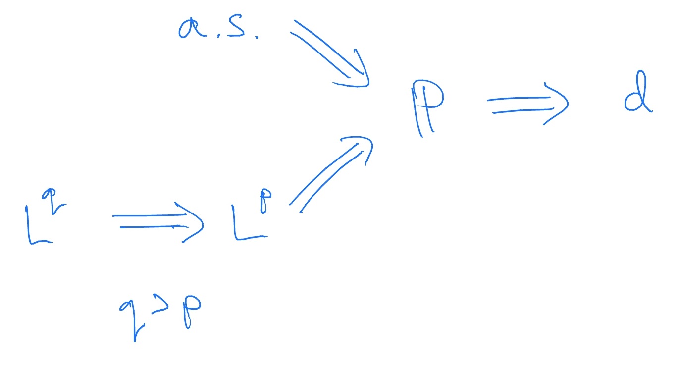
4. Let \(1\leq p< q\). If \(X_n\stackrel {L^q}{\to } X\) then \(X_n\stackrel {L^p}{\to } X\).
In all other cases (i.e. that are not automatically implied by the above), convergence in one mode does not imply convergence in another.
-
The proofs are not part of our course (they are part of MAS31002/61022). We can summarise Lemma 6.1.2 with a diagram:
-
Remark 6.1.3 For convergence of real numbers, it was shown in MAS221 that if \(a_n\to a\) and \(a_n\to b\) then \(a=b\), which is known as uniqueness of limits. For random variables, the situation is a little more complicated: if \(X_n\stackrel {\P }{\to } X\) and \(X_n\stackrel {\P }{\to } Y\) then \(X=Y\) almost surely. By Lemma 6.1.2, this result also applies to \(\stackrel {L^p}{\to }\) and \(\stackrel {a.s.}{\to }\). However, if we have only \(X_n\stackrel {d}{\to } X\) and \(X_n\stackrel {d}{\to } Y\) then we can only conclude that \(X\) and \(Y\) have the same distribution function. Proving these facts is one of the challenge exercises, 6.6.