Stochastic Processes and Financial Mathematics
(part one)

$\newcommand{\footnotename}{footnote}$ $\def \LWRfootnote {1}$ $\newcommand {\footnote }[2][\LWRfootnote ]{{}^{\mathrm {#1}}}$ $\newcommand {\footnotemark }[1][\LWRfootnote ]{{}^{\mathrm {#1}}}$ $\let \LWRorighspace \hspace $ $\renewcommand {\hspace }{\ifstar \LWRorighspace \LWRorighspace }$ $\newcommand {\mathnormal }[1]{{#1}}$ $\newcommand \ensuremath [1]{#1}$ $\newcommand {\LWRframebox }[2][]{\fbox {#2}} \newcommand {\framebox }[1][]{\LWRframebox } $ $\newcommand {\setlength }[2]{}$ $\newcommand {\addtolength }[2]{}$ $\newcommand {\setcounter }[2]{}$ $\newcommand {\addtocounter }[2]{}$ $\newcommand {\arabic }[1]{}$ $\newcommand {\number }[1]{}$ $\newcommand {\noalign }[1]{\text {#1}\notag \\}$ $\newcommand {\cline }[1]{}$ $\newcommand {\directlua }[1]{\text {(directlua)}}$ $\newcommand {\luatexdirectlua }[1]{\text {(directlua)}}$ $\newcommand {\protect }{}$ $\def \LWRabsorbnumber #1 {}$ $\def \LWRabsorbquotenumber "#1 {}$ $\newcommand {\LWRabsorboption }[1][]{}$ $\newcommand {\LWRabsorbtwooptions }[1][]{\LWRabsorboption }$ $\def \mathchar {\ifnextchar "\LWRabsorbquotenumber \LWRabsorbnumber }$ $\def \mathcode #1={\mathchar }$ $\let \delcode \mathcode $ $\let \delimiter \mathchar $ $\def \oe {\unicode {x0153}}$ $\def \OE {\unicode {x0152}}$ $\def \ae {\unicode {x00E6}}$ $\def \AE {\unicode {x00C6}}$ $\def \aa {\unicode {x00E5}}$ $\def \AA {\unicode {x00C5}}$ $\def \o {\unicode {x00F8}}$ $\def \O {\unicode {x00D8}}$ $\def \l {\unicode {x0142}}$ $\def \L {\unicode {x0141}}$ $\def \ss {\unicode {x00DF}}$ $\def \SS {\unicode {x1E9E}}$ $\def \dag {\unicode {x2020}}$ $\def \ddag {\unicode {x2021}}$ $\def \P {\unicode {x00B6}}$ $\def \copyright {\unicode {x00A9}}$ $\def \pounds {\unicode {x00A3}}$ $\let \LWRref \ref $ $\renewcommand {\ref }{\ifstar \LWRref \LWRref }$ $ \newcommand {\multicolumn }[3]{#3}$ $\require {textcomp}$ $\newcommand {\intertext }[1]{\text {#1}\notag \\}$ $\let \Hat \hat $ $\let \Check \check $ $\let \Tilde \tilde $ $\let \Acute \acute $ $\let \Grave \grave $ $\let \Dot \dot $ $\let \Ddot \ddot $ $\let \Breve \breve $ $\let \Bar \bar $ $\let \Vec \vec $ $\DeclareMathOperator {\var }{var}$ $\DeclareMathOperator {\cov }{cov}$ $\def \ra {\Rightarrow }$ $\def \to {\rightarrow }$ $\def \iff {\Leftrightarrow }$ $\def \sw {\subseteq }$ $\def \wt {\widetilde }$ $\def \mc {\mathcal }$ $\def \mb {\mathbb }$ $\def \sc {\setminus }$ $\def \v {\textbf }$ $\def \p {\partial }$ $\def \E {\mb {E}}$ $\def \P {\mb {P}}$ $\def \R {\mb {R}}$ $\def \C {\mb {C}}$ $\def \N {\mb {N}}$ $\def \Q {\mb {Q}}$ $\def \Z {\mb {Z}}$ $\def \B {\mb {B}}$ $\def \~{\sim }$ $\def \-{\,;\,}$ $\def \|{\,|\,}$ $\def \qed {$\blacksquare $}$ $\def \1{\unicode {x1D7D9}}$ $\def \cadlag {c\`{a}dl\`{a}g}$ $\def \p {\partial }$ $\def \l {\left }$ $\def \r {\right }$ $\def \F {\mc {F}}$ $\def \G {\mc {G}}$ $\def \H {\mc {H}}$ $\def \Om {\Omega }$ $\def \om {\omega }$

5.6 Hedging

We can adapt the derivatives from Section 5.3 to the binomial model, by simply replacing time $1$ with time $T$. For example, in the binomial model a forward contract is the obligation to buy a single unit of stock at time $T$ for a strike price $K$ that is agreed at time $0$.

Definition 5.6.1 A contingent claim is a random variable of the form $\Phi (S_T)$, where $\Phi :\R \to \R $ is a deterministic function.

For a forward contract, the contingent claim would be $\Phi (S_T)=S_T-K$.

Definition 5.6.2 We say that a portfolio strategy $h=(h_t)_{t=1}^T$ is a replicating portfolio or hedging strategy for the contingent claim $\Phi (S_T)$ if $h$ is self-financing and $V^h_T=\Phi (S_T)$.

These match the definitions for the one-period model, except we now care about the value of the asset at time $T$ (instead of time $1$). We will shortly look at how to find replicating portfolios.

As in the one-period model, the binomial model is said to be complete if every contingent claim can be replicated. Further, as in the one-period model, if the binomial model is free of arbitrage then it is also complete. With this in mind, for the rest of this section we assume that

\[d<1+r<u.\]

Lastly, as in the one-period model, our assumption that there is no arbitrage means that:

If a contingent claim $\Phi (S_T)$ has a replicating portfolio $h=(h_t)_{t=1}^T$, then the price of the $\Phi (S_T)$ at time $0$ must be equal to the value of $h_0$.

Now, let us end this chapter by showing how to compute prices and replicating portfolios in the binomial model. We already know how to do this in the one-period model, see Example 5.2.4. We could do it in full generality (as we did in (5.7) for the one-period model) but this would involve lots of indices and look rather messy. Instead, we’ll work through a practical example that makes the general strategy clear.

Let us take $T=3$ and set

\[S_0=80,\quad u=1.5,\quad d=0.5,\quad p_u=0.6,\quad p_d=0.4.\]

To make the calculations easier, we’ll also take our interest rate to be $r=0$. We’ll price a European call option with strike price $K=80$. The contingent claim for this option, which is

\begin{equation} \label {eq:eco_ex} \Phi (S_T)=\max (S_T-K,0). \end{equation}

STEP 1 is to work our the risk-neutral probabilities. From (5.3), these are $q_u=\frac {1+0-0.5}{1.5-0.5}=0.5$ and $q_d=1-q_u=0.5$.

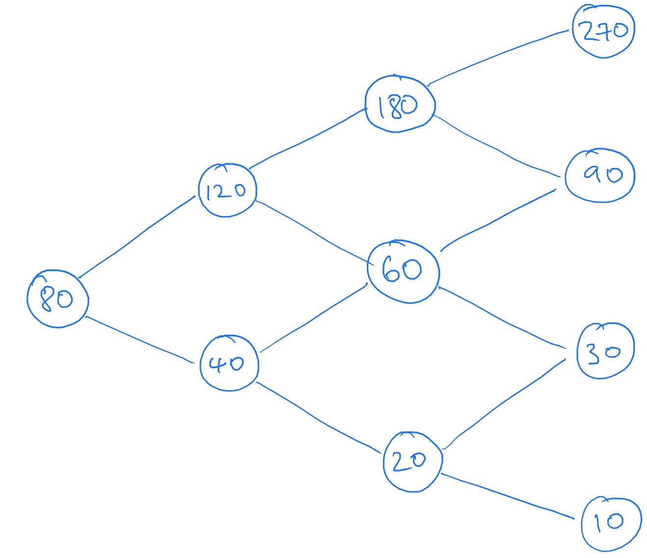
STEP 2 is to write down the tree of possible values that the stock can take during time $t=0,1,2,3$. This looks like

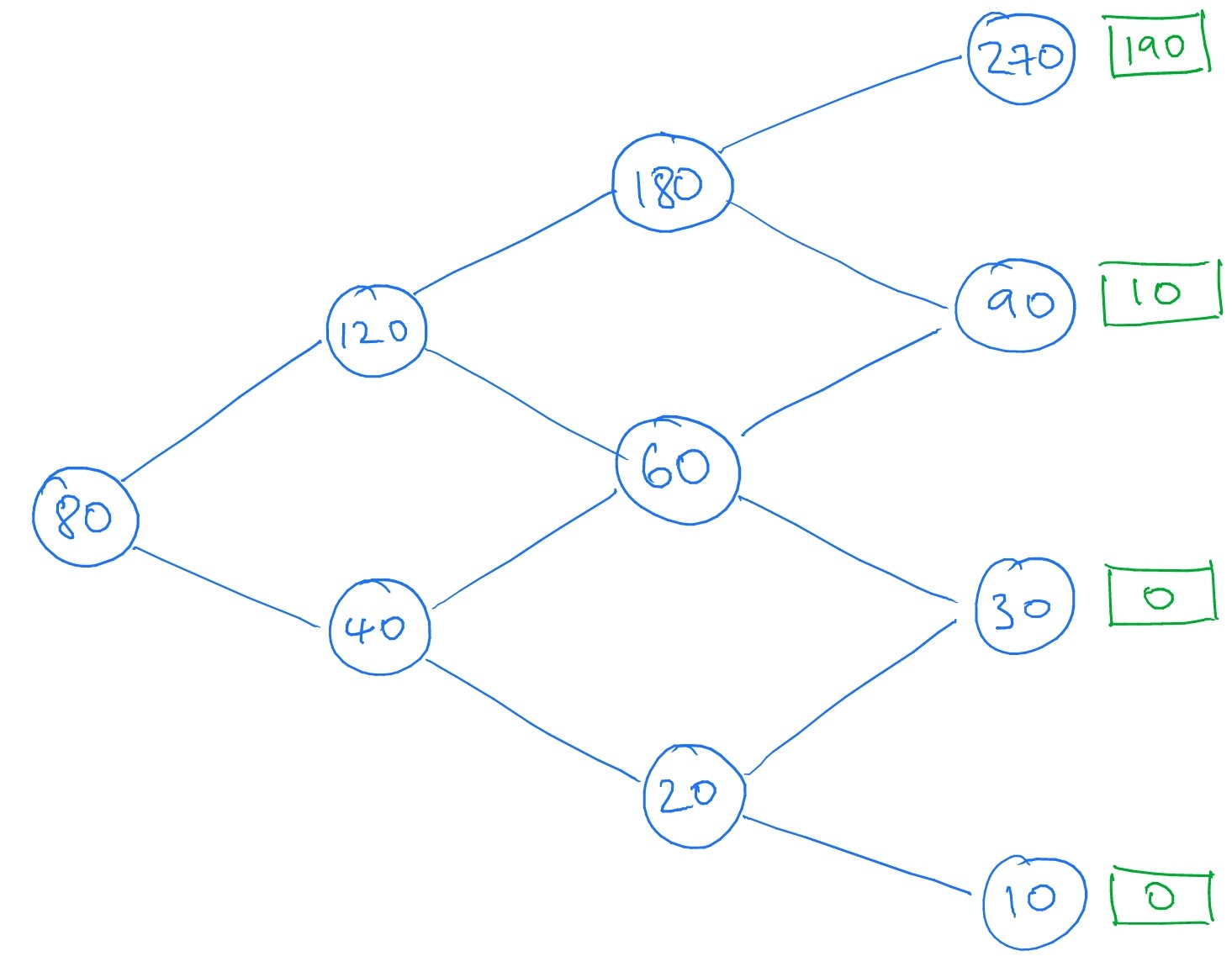
We then work out, at each of the nodes corresponding to time $T=3$, what the value of our contingent claim (5.10) would be if this node were reached. We write these values in square boxes:

We now come to STEP 3, the key idea. Suppose we are sitting in one of the nodes at time $t=2$, which we think of as the ‘current’ node. For example suppose we are at the uppermost node (labelled $180$, the ‘current’ value of the stock). Looking forwards one step of time we can see that, if the stock price goes up our option is worth $190$, whereas if the stock price goes down our option is worth $10$. What we are seeing here is (an instance of) the one-period model! With contingent claim

\[\wt \Phi (su)=190,\quad \wt \Phi (sd)=10.\]

So, using the one-period risk-neutral valuation formula from Proposition 5.2.6 the value of our call option at our current node is

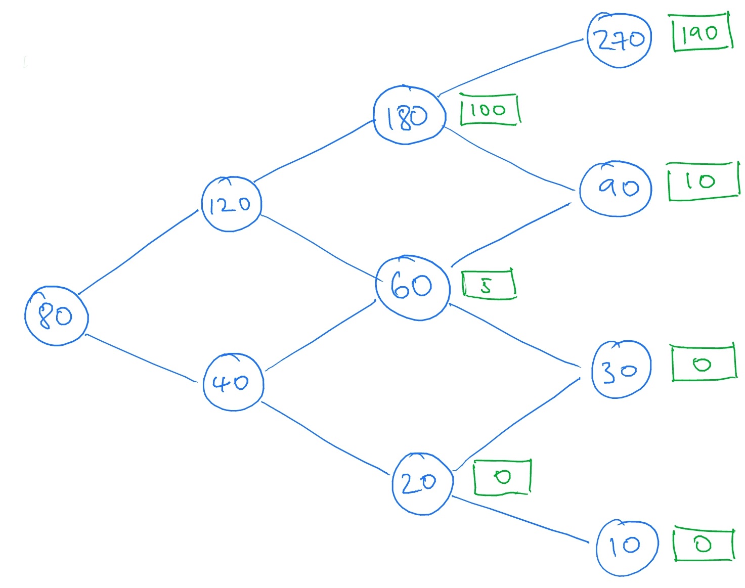
\[\frac {1}{1+0}(190\cdot 0.5+10\cdot 0.5)=100.\]

We could apply the same logic to any of the nodes corresponding to time $t=2$, and compute the value of our call option at that node:

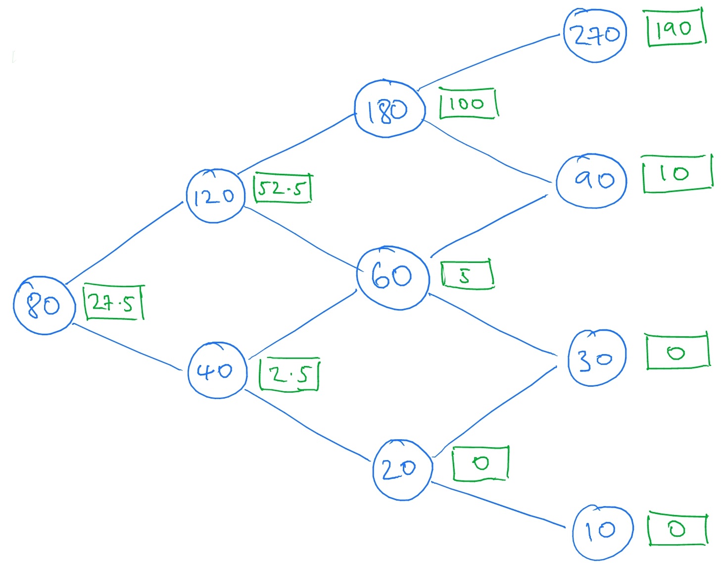
If we now imagine ourselves sitting in one of the nodes at time $t=1$, and look forwards one step in time, we again find ourselves faced with an instance of the one-period model. This allows us to compute the value of our call option at the $t=1$ nodes; take for example the node labelled by $40$ which, one step into the future, sees the contingent claim $\wt \Phi (su)=5, \wt \Phi (sd)=0$ and using $\eqref {eq:risk_free}$ gives the value of the call option at this node as $\frac {1}{1+0}(5\times 0.5+0\times 0.5)=2.5$. Repeating the procedure on the other $t=1$ node, and then also on the single $t=0$ node gives us

Therefore, the value (i.e. the price) of our call option at time $t=0$ is $27.5$.

Although we have computed the price, we haven’t yet computed a replicating portfolio, which is STEP 4. We could do it by solving lots of linear equations for our one-period models, as in Example 5.2.4, but since we have several steps a quicker way is to apply Proposition 5.2.6 and use the general formula we found in (5.8).

Starting at time $t=0$, to replicate the contingent claim $\wt \Phi (su)=52.5$ and $\wt \Phi (sd)=2.5$ at time $t=1$, equation (5.8) tells us that we want the portfolio

\[x_1=\frac {1}{1+0}\frac {1.5\cdot 2.5-0.5\cdot 52.5}{1.5-0.5}=-22.5,\quad y_1=\frac {1}{80}\frac {52.5-2.5}{1.5-0.5}=\frac {5}{8}.\]

The value of this portfolio at time $0$ is

\[x_1+80y_1=-22.5+80\cdot \frac 58=27.5\]

which is equal to the initial value of our call option.

We can then carry on forwards. For example, if the stock went up in between $t=0$ and $t=1$, then at time $t=1$ we would be sitting in the node for $S_1=120$, labelled simply $120$. Our portfolio $(x_1,y_1)$ is now worth

\[x_1(1+0)+y_1\cdot 120=-22.5+120\cdot \frac 58=52.5,\]

equal to what is now the value of our call option. We use (5.8) again to calculate the portfolio we want to hold during time $1\mapsto 2$, this time with $\wt \Phi (su)=100$ and $\wt \Phi (sd)=5$, giving $x_2=-42.5$ and $y_2=\frac {95}{120}.$ You can check that the current value of the portfolio $(x_2,y_2)$ is $52.5$.

Next, suppose the stock price falls between $t=1$ and $t=2$, so our next node is $S_2=60$. Our portfolio $(x_2,y_2)$ now becomes worth

\[x_2(1+0)+y_2\cdot 60 = -42.5+\frac {95}{120}\cdot 60 = 5,\]

again equal to the value our of call option. For the final step, we must replicate the contingent claim $\wt \Phi (su)=10$, $\wt \Phi (sd)=0$, which (5.8) tells us is done using $x_3=-5$ and $y_3=\frac {1}{6}.$ Again, you can check that the current value of this portfolio is $5$.

Lastly, the stock price rises again to $S_3=90$. Our portfolio becomes worth

\[x_3(1+0)+y_3\cdot 90 = -5+\frac {1}{6}\cdot 90 = 10,\]

equal to the payoff from our call option.

To sum up, using (5.8) we can work out which portfolio we would want to hold, at each possible outcome of the stock changing value. At all times we would be holding a portfolio with current value equal to the current value of the call option. Therefore, this gives a self-financing portfolio strategy that replicates $\Phi (S_T)$.

Stochastic Processes and Financial Mathematics (part one)

5.6 Hedging

Stochastic Processes and Financial Mathematics
(part one)