Stochastic Processes and Financial Mathematics
(part one)

Chapter 4 Stochastic processes

In this chapter we introduce stochastic processes, with a selection of examples that are commonly used as building blocks in stochastic modelling. We show that these stochastic processes are closely connected to martingales.

For example, a sequence of i.i.d. random variables is a stochastic process. A martingale is a stochastic process. A Markov chain (from MAS2003, for those who took it) is a stochastic process. And so on.

For any stochastic process \((X_n)\) the natural or generated filtration of \((X_n)\) is the filtration given by

\[\mc {F}_n=\sigma (X_1,X_2,\ldots ,X_n).\]

Therefore, a random variable is \(\mc {F}_m\) measurable if it depends only on the behaviour of our stochastic process up until time \(m\).

From now on we adopt the convention (which is standard in the field of stochastic processes) that whenever we don’t specify a filtration explicitly we mean to use the generated filtration.

4.1 Random walks

Random walks are stochastic processes that ‘walk around’ in space. We think of a particle that moves between vertices of \(\Z \). At each step of time, the particle chooses at random to either move up or down, for example from \(x\) to \(x+1\) or \(x-1\).

Simple symmetric random walk

Let \((X_i)_{i=1}^\infty \) be a sequence of i.i.d. random variables where

\begin{equation} \label {eq:srw_step} \P [X_i=1]=\P [X_i=-1]=\frac {1}{2}. \end{equation}

The simple symmetric random walk is the stochastic process

\[S_n=\sum \limits _{i=1}^n X_i.\]

By convention, this means that \(S_0=0\). The word ‘simple’ refers to the fact that the walk moves by precisely \(1\) unit of space in each step of time i.e. \(|X_i|=1\). A sample path of \(S_n\), which means a sample of the sequence \((S_0,S_1,S_2,\ldots )\), might look like:

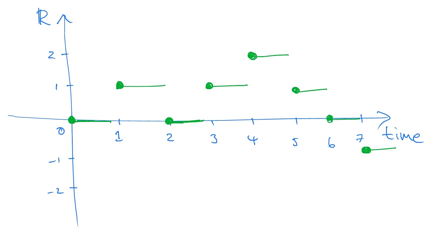
Note that when time is discrete \(t=0,1,2,\ldots \) it is standard to draw the location of the random walk (and other stochastic processes) as constant in between integer time points.

Because of (4.1), the random walk is equally likely to move upwards or downwards. This case is known as the ‘symmetric’ random walk because, if \(S_0=0\), the two stochastic processes \(S_n\) and \(-S_n\) have the same distribution.

We have already seen (in Section 3.3) that \(S_n\) is a martingale, with respect to its generated filtration

\[\mc {F}_n=\sigma (X_1,\ldots ,X_n)=\sigma (S_1,\ldots ,S_n).\]

It should seem very natural that \((S_n)\) is a martingale – going upwards as much as downwards is ‘fair’.

Simple asymmetric random walk

Let \((X_i)_{i=1}^\infty \) be a sequence of i.i.d. random variables. Let \(p+q=1\) with \(p,q\in [0,1]\), \(p\neq q\) and suppose that

\[\P [X_i=1]=p,\hspace {1pc}\P [X_i=-1]=q.\]

The asymmetric random walk is the stochastic process

\[S_n=\sum \limits _{i=1}^n X_i.\]

The key difference to the symmetric random walk is that here we have \(p\neq q\) (the symmetric random walk has \(p=q=\frac 12\)). The asymmetric random walk is more likely to step upwards than downwards if \(p>q\), and vice versa if \(q<p\). The technical term for this behaviour is drift. A sample path for the case \(p>q\) might look like:

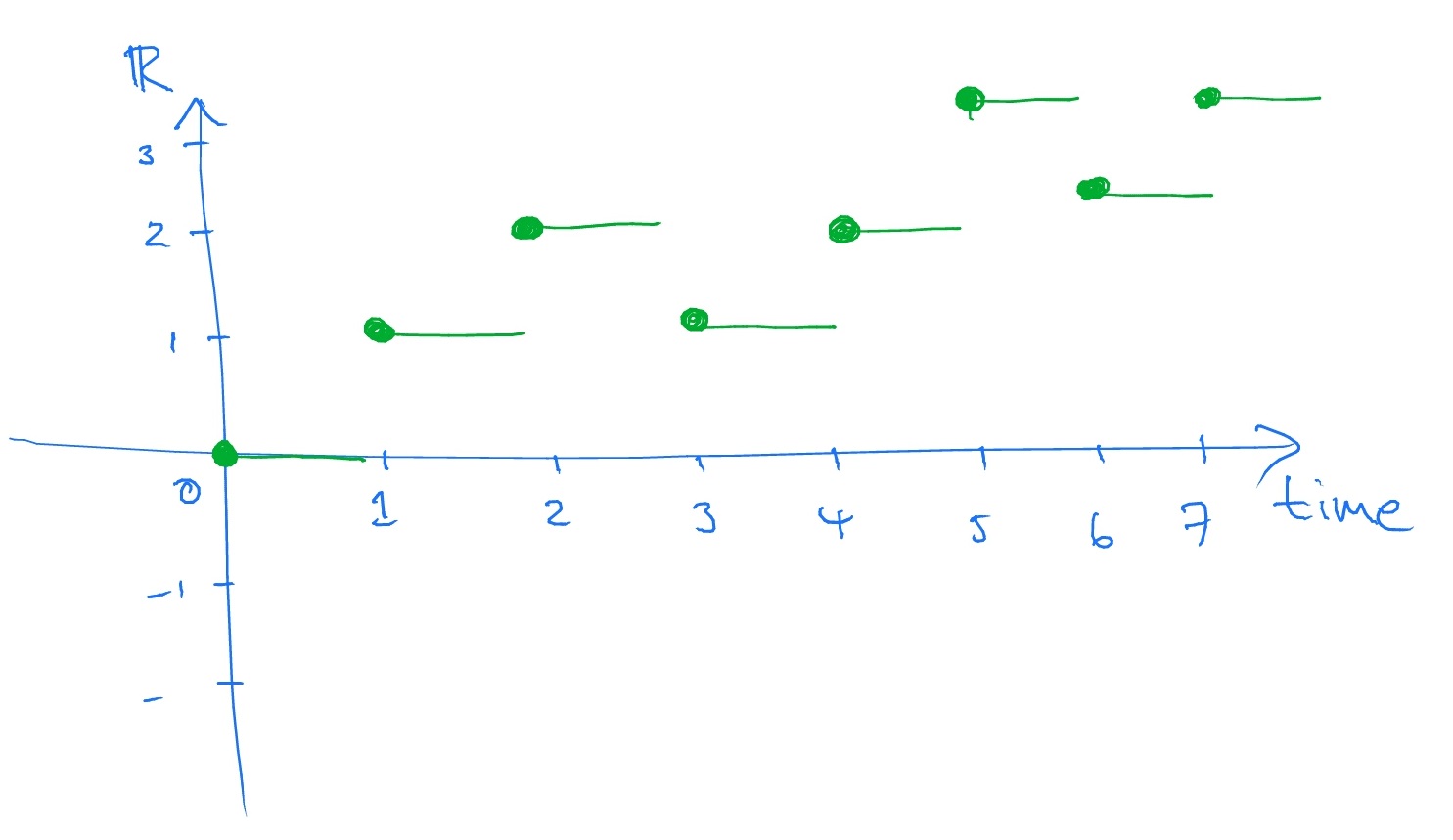
This is ‘unfair’, because of the drift upwards, so we should suspect that the asymmetric random walk is not a martingale. In fact,

\begin{equation} \label {eq:rw_drift} \E [S_n]=\sum \limits _{i=1}^n\E [X_i]=\sum \limits _{i=1}^n(p-q)=n(p-q), \end{equation}

whereas \(\E [S_0]=0\). Thus, Lemma 3.3.6 confirms that \(S_n\) is not a martingale. However, the process

\begin{equation} \label {eq:drift_compensate} M_n=S_n-n(p-q) \end{equation}

is a martingale. The key is that the term \(n(p-q)\) compensates for the drift and ‘restores fairness’.

We’ll now prove that \((M_n)\) is a martingale. Since \(X_i\in m\mc {F}_n\) for all \(i\leq n\), by Proposition 2.2.6 we have \(S_n-n(p-q)\in m\mc {F}_n\). Since \(|X_i|\leq 1\) we have

\[|S_n-n(p-q)|\leq |S_n|+n|p-q|\leq n+n|p-q|\]

and hence \(M_n\) is bounded, so \(M_n\in L^1\). Lastly,

\begin{align*} \E [S_{n+1}-(n+1)(p-q)\|\mc {F}_n] &=\E [S_{n+1}\|\mc {F}_n]-(n+1)(p-q)\\ &=\E [X_{n+1}\|\mc {F}_n]+\E [S_n\|\mc {F}_n]-(n+1)(p-q)\\ &=\E [X_{n+1}]+S_n-(n+1)(p-q)\\ &=(p-q)+S_n-(n+1)(p-q)\\ &=S_n-n(p-q). \end{align*} Therefore \(\E [M_{n+1}\|\mc {F}_n]=M_n\), and \((M_n)\) is a martingale.