Stochastic Processes and Financial Mathematics
(part one)
\(\newcommand{\footnotename}{footnote}\)
\(\def \LWRfootnote {1}\)
\(\newcommand {\footnote }[2][\LWRfootnote ]{{}^{\mathrm {#1}}}\)
\(\newcommand {\footnotemark }[1][\LWRfootnote ]{{}^{\mathrm {#1}}}\)
\(\let \LWRorighspace \hspace \)
\(\renewcommand {\hspace }{\ifstar \LWRorighspace \LWRorighspace }\)
\(\newcommand {\mathnormal }[1]{{#1}}\)
\(\newcommand \ensuremath [1]{#1}\)
\(\newcommand {\LWRframebox }[2][]{\fbox {#2}} \newcommand {\framebox }[1][]{\LWRframebox } \)
\(\newcommand {\setlength }[2]{}\)
\(\newcommand {\addtolength }[2]{}\)
\(\newcommand {\setcounter }[2]{}\)
\(\newcommand {\addtocounter }[2]{}\)
\(\newcommand {\arabic }[1]{}\)
\(\newcommand {\number }[1]{}\)
\(\newcommand {\noalign }[1]{\text {#1}\notag \\}\)
\(\newcommand {\cline }[1]{}\)
\(\newcommand {\directlua }[1]{\text {(directlua)}}\)
\(\newcommand {\luatexdirectlua }[1]{\text {(directlua)}}\)
\(\newcommand {\protect }{}\)
\(\def \LWRabsorbnumber #1 {}\)
\(\def \LWRabsorbquotenumber "#1 {}\)
\(\newcommand {\LWRabsorboption }[1][]{}\)
\(\newcommand {\LWRabsorbtwooptions }[1][]{\LWRabsorboption }\)
\(\def \mathchar {\ifnextchar "\LWRabsorbquotenumber \LWRabsorbnumber }\)
\(\def \mathcode #1={\mathchar }\)
\(\let \delcode \mathcode \)
\(\let \delimiter \mathchar \)
\(\def \oe {\unicode {x0153}}\)
\(\def \OE {\unicode {x0152}}\)
\(\def \ae {\unicode {x00E6}}\)
\(\def \AE {\unicode {x00C6}}\)
\(\def \aa {\unicode {x00E5}}\)
\(\def \AA {\unicode {x00C5}}\)
\(\def \o {\unicode {x00F8}}\)
\(\def \O {\unicode {x00D8}}\)
\(\def \l {\unicode {x0142}}\)
\(\def \L {\unicode {x0141}}\)
\(\def \ss {\unicode {x00DF}}\)
\(\def \SS {\unicode {x1E9E}}\)
\(\def \dag {\unicode {x2020}}\)
\(\def \ddag {\unicode {x2021}}\)
\(\def \P {\unicode {x00B6}}\)
\(\def \copyright {\unicode {x00A9}}\)
\(\def \pounds {\unicode {x00A3}}\)
\(\let \LWRref \ref \)
\(\renewcommand {\ref }{\ifstar \LWRref \LWRref }\)
\( \newcommand {\multicolumn }[3]{#3}\)
\(\require {textcomp}\)
\(\newcommand {\intertext }[1]{\text {#1}\notag \\}\)
\(\let \Hat \hat \)
\(\let \Check \check \)
\(\let \Tilde \tilde \)
\(\let \Acute \acute \)
\(\let \Grave \grave \)
\(\let \Dot \dot \)
\(\let \Ddot \ddot \)
\(\let \Breve \breve \)
\(\let \Bar \bar \)
\(\let \Vec \vec \)
\(\DeclareMathOperator {\var }{var}\)
\(\DeclareMathOperator {\cov }{cov}\)
\(\def \ra {\Rightarrow }\)
\(\def \to {\rightarrow }\)
\(\def \iff {\Leftrightarrow }\)
\(\def \sw {\subseteq }\)
\(\def \wt {\widetilde }\)
\(\def \mc {\mathcal }\)
\(\def \mb {\mathbb }\)
\(\def \sc {\setminus }\)
\(\def \v {\textbf }\)
\(\def \p {\partial }\)
\(\def \E {\mb {E}}\)
\(\def \P {\mb {P}}\)
\(\def \R {\mb {R}}\)
\(\def \C {\mb {C}}\)
\(\def \N {\mb {N}}\)
\(\def \Q {\mb {Q}}\)
\(\def \Z {\mb {Z}}\)
\(\def \B {\mb {B}}\)
\(\def \~{\sim }\)
\(\def \-{\,;\,}\)
\(\def \|{\,|\,}\)
\(\def \qed {$\blacksquare $}\)
\(\def \1{\unicode {x1D7D9}}\)
\(\def \cadlag {c\`{a}dl\`{a}g}\)
\(\def \p {\partial }\)
\(\def \l {\left }\)
\(\def \r {\right }\)
\(\def \F {\mc {F}}\)
\(\def \G {\mc {G}}\)
\(\def \H {\mc {H}}\)
\(\def \Om {\Omega }\)
\(\def \om {\omega }\)
5.4 The binomial model
Let us step back and examine our progress, for a moment. We now know about as much about one-period model as there is to know. It is time to move onto to a more complicated (and more realistic) model. The
one-period model is unsatisfactory in two main respects:
We’ll start to address the first of these points now. The second point waits until the second semester of the course.
Adding multiple time steps to our model will make use of the theory we developed in Chapters 2 and 3. It will also reveal a surprising connection between arbitrage and martingales.
The binomial model has time points \(t=0,1,2,\ldots ,T\). Inside each time step, we have a single step of the one-period model. This means that cash earns interest at rate \(r\):
For our stock, we’ll have to think a little harder. In a single time step, the value of our stock is multiplied by a random variable \(Z\) with distribution \(\P [Z=u]=p_u\), \(\P [Z=d]=p_d\). We now have several
time steps. For each time step we’ll use a new independent \(Z\). So, let \((Z_t)_{t=1}^{T}\) be a sequence of i.i.d. random variables each with the distribution of \(Z\).
-
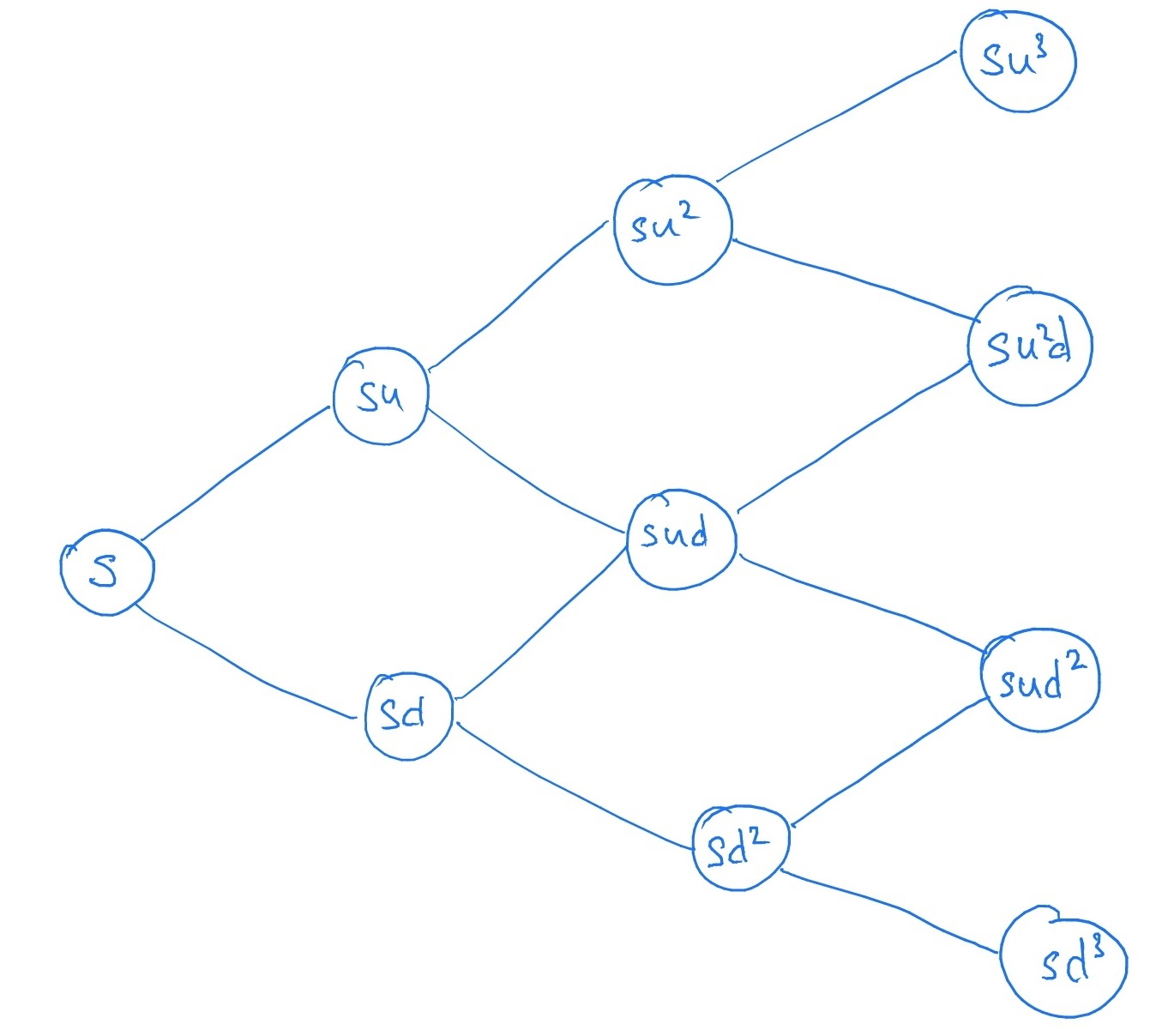
• The value of a single unit of stock at time \(t\) is given by
\(\seteqnumber{0}{5.}{9}\)
\begin{align*}
S_0&=s,\\ S_{t}&=Z_{t}S_{t-1}.
\end{align*}
We can illustrate the process \((S_t)\) using a tree-like diagram:
Note that the tree is recombining, in the sense that a move up (by \(u\)) followed by a move down (by \(d\)) has the same outcome as a move down followed by a move up. It’s like a random walk, except we
multiply instead of add (recall exercise 4.1).