Stochastic Processes and Financial Mathematics
(part two)

$\newcommand{\footnotename}{footnote}$ $\def \LWRfootnote {1}$ $\newcommand {\footnote }[2][\LWRfootnote ]{{}^{\mathrm {#1}}}$ $\newcommand {\footnotemark }[1][\LWRfootnote ]{{}^{\mathrm {#1}}}$ $\let \LWRorighspace \hspace $ $\renewcommand {\hspace }{\ifstar \LWRorighspace \LWRorighspace }$ $\newcommand {\mathnormal }[1]{{#1}}$ $\newcommand \ensuremath [1]{#1}$ $\newcommand {\LWRframebox }[2][]{\fbox {#2}} \newcommand {\framebox }[1][]{\LWRframebox } $ $\newcommand {\setlength }[2]{}$ $\newcommand {\addtolength }[2]{}$ $\newcommand {\setcounter }[2]{}$ $\newcommand {\addtocounter }[2]{}$ $\newcommand {\arabic }[1]{}$ $\newcommand {\number }[1]{}$ $\newcommand {\noalign }[1]{\text {#1}\notag \\}$ $\newcommand {\cline }[1]{}$ $\newcommand {\directlua }[1]{\text {(directlua)}}$ $\newcommand {\luatexdirectlua }[1]{\text {(directlua)}}$ $\newcommand {\protect }{}$ $\def \LWRabsorbnumber #1 {}$ $\def \LWRabsorbquotenumber "#1 {}$ $\newcommand {\LWRabsorboption }[1][]{}$ $\newcommand {\LWRabsorbtwooptions }[1][]{\LWRabsorboption }$ $\def \mathchar {\ifnextchar "\LWRabsorbquotenumber \LWRabsorbnumber }$ $\def \mathcode #1={\mathchar }$ $\let \delcode \mathcode $ $\let \delimiter \mathchar $ $\def \oe {\unicode {x0153}}$ $\def \OE {\unicode {x0152}}$ $\def \ae {\unicode {x00E6}}$ $\def \AE {\unicode {x00C6}}$ $\def \aa {\unicode {x00E5}}$ $\def \AA {\unicode {x00C5}}$ $\def \o {\unicode {x00F8}}$ $\def \O {\unicode {x00D8}}$ $\def \l {\unicode {x0142}}$ $\def \L {\unicode {x0141}}$ $\def \ss {\unicode {x00DF}}$ $\def \SS {\unicode {x1E9E}}$ $\def \dag {\unicode {x2020}}$ $\def \ddag {\unicode {x2021}}$ $\def \P {\unicode {x00B6}}$ $\def \copyright {\unicode {x00A9}}$ $\def \pounds {\unicode {x00A3}}$ $\let \LWRref \ref $ $\renewcommand {\ref }{\ifstar \LWRref \LWRref }$ $ \newcommand {\multicolumn }[3]{#3}$ $\require {textcomp}$ $\newcommand {\intertext }[1]{\text {#1}\notag \\}$ $\let \Hat \hat $ $\let \Check \check $ $\let \Tilde \tilde $ $\let \Acute \acute $ $\let \Grave \grave $ $\let \Dot \dot $ $\let \Ddot \ddot $ $\let \Breve \breve $ $\let \Bar \bar $ $\let \Vec \vec $ $\DeclareMathOperator {\var }{var}$ $\DeclareMathOperator {\cov }{cov}$ $\DeclareMathOperator {\indeg }{deg_{in}}$ $\DeclareMathOperator {\outdeg }{deg_{out}}$ $\newcommand {\nN }{n \in \mathbb {N}}$ $\newcommand {\Br }{{\cal B}(\R )}$ $\newcommand {\F }{{\cal F}}$ $\newcommand {\ds }{\displaystyle }$ $\newcommand {\st }{\stackrel {d}{=}}$ $\newcommand {\uc }{\stackrel {uc}{\rightarrow }}$ $\newcommand {\la }{\langle }$ $\newcommand {\ra }{\rangle }$ $\newcommand {\li }{\liminf _{n \rightarrow \infty }}$ $\newcommand {\ls }{\limsup _{n \rightarrow \infty }}$ $\newcommand {\limn }{\lim _{n \rightarrow \infty }}$ $\def \ra {\Rightarrow }$ $\def \to {\rightarrow }$ $\def \iff {\Leftrightarrow }$ $\def \sw {\subseteq }$ $\def \wt {\widetilde }$ $\def \mc {\mathcal }$ $\def \mb {\mathbb }$ $\def \sc {\setminus }$ $\def \v {\textbf }$ $\def \p {\partial }$ $\def \E {\mb {E}}$ $\def \P {\mb {P}}$ $\def \R {\mb {R}}$ $\def \C {\mb {C}}$ $\def \N {\mb {N}}$ $\def \Q {\mb {Q}}$ $\def \Z {\mb {Z}}$ $\def \B {\mb {B}}$ $\def \~{\sim }$ $\def \-{\,;\,}$ $\def \|{\,|\,}$ $\def \qed {$\blacksquare $}$ $\def \1{\unicode {x1D7D9}}$ $\def \cadlag {c\`{a}dl\`{a}g}$ $\def \p {\partial }$ $\def \l {\left }$ $\def \r {\right }$ $\def \F {\mc {F}}$ $\def \G {\mc {G}}$ $\def \H {\mc {H}}$ $\def \Om {\Omega }$ $\def \om {\omega }$ $\def \Vega {\mc {V}}$

Chapter 11 Brownian motion

In this chapter we study the most important example of a stochastic process: Brownian motion. In essence, Brownian motion is the continuous time equivalent of the symmetric random walk that we studied in Section 4.1.

11.1 The limit of random walks

The discovery of Brownian motion has a distinguished place in the history of both science and mathematics. As with most great discoveries in the scientific world, many people discovered parts of what later became known as Brownian motion, using varying degrees of mathematical and experimental precision, at around the same time.

Brownian motion is named after the botanist Robert Brown who, in 1827, through a microscope, saw erratic movements being made by tiny pollen organelles floating on water. The cause of these movements was explained later by Albert Einstein and the physicist Jean Perrin: the movements were caused by (the cumulative effect of) many individual water molecules hitting the tiny organelles. This realization provided the ‘modern science’ of the time with a key piece of evidence for the existence of atoms¹. Around the same time, the american mathematician Norbert Wiener, building on earlier work of Louis Bachelier, developed a mathematical model for stock prices and independently discovered Brownian motion.

Today, Brownian motion is at the heart of many important models of the physical world. We will see some examples in future sections of the course; for now our first task is to construct the process.

Brown, Einstein and Perrin studied pollen movements on the surface of still water, meaning they observed movements in two (spatial) dimensions $\R ^2$. Bachelier, by contrast, saw stocks prices moving up and down - in one dimension $\R $. In both cases the underlying principle is one of ‘completely random’ movement. We will restrict to the one dimensional case in this course.

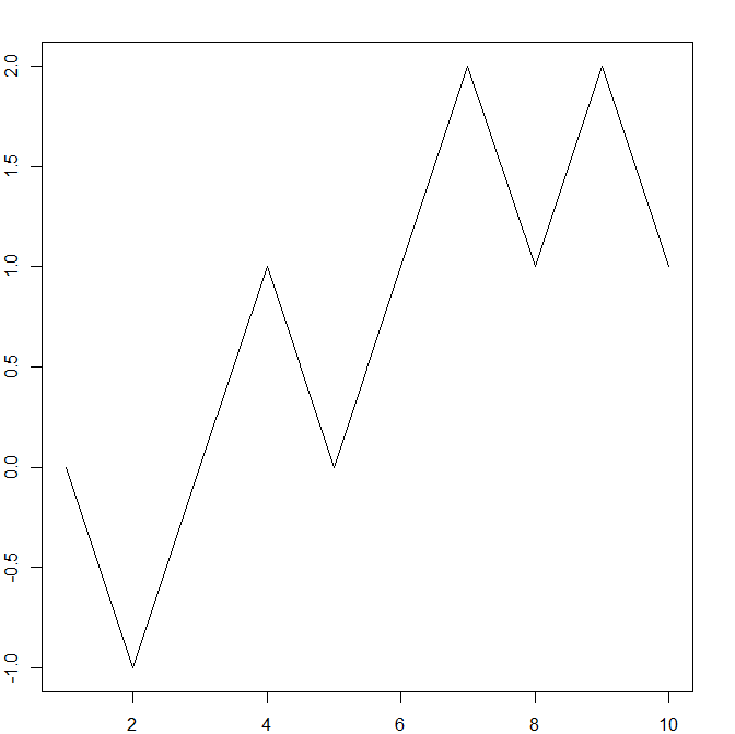
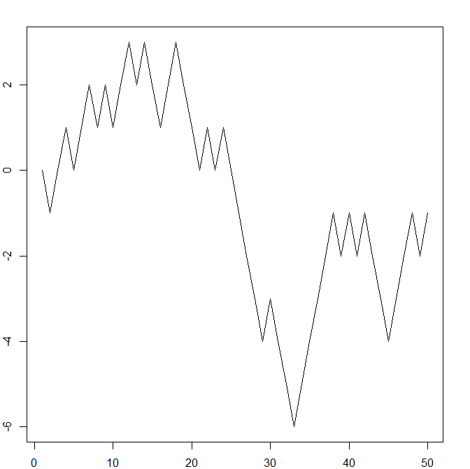
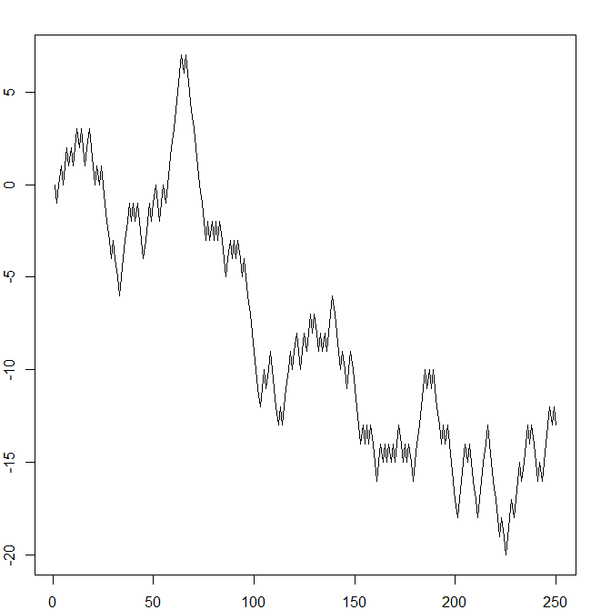
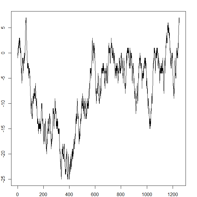
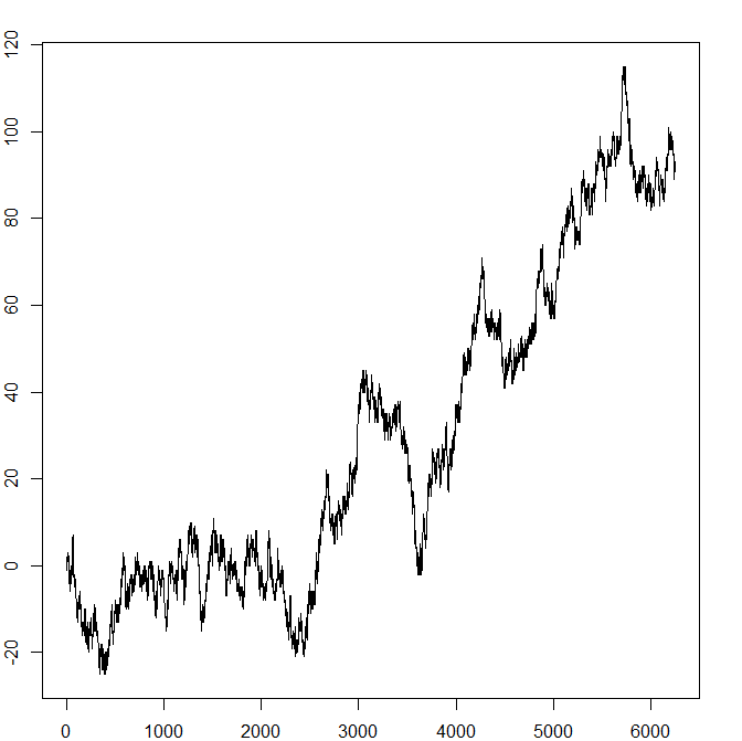
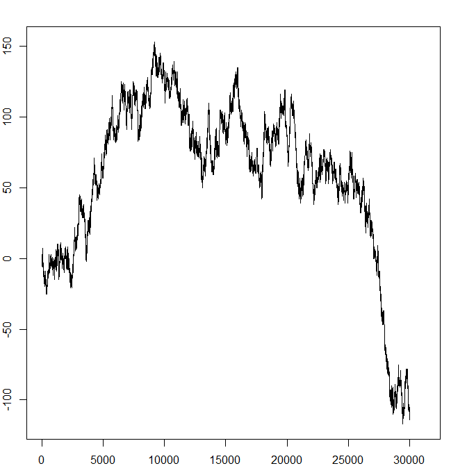
Recall the symmetric random walk from Section 4.1. We will look at six pictures of (samples of) it, where in each picture the random walk has run for a successively longer time ($T=10,50,250,1250,6250,31250$). We fit each such picture into the same size box – we can think of this as zooming out, so in each inch of space on the paper we see more and more, smaller and smaller, jumps of the random walk. The results are intriguing:

.

As we zoom out further and further, the pictures are starting to look very similar in character. The last three are all ‘jagged’ in a conspicuously similar way. If you look carefully, you can see that each picture contains precisely the first fifth (in terms of time passed) of the next picture. From the axis on pictures, we might guess that, if we have $T$ units of time on the $x$-axis, we need about $\sqrt {T}$ units of space on the $y$-axis. This is not surprising: a short calculation (which we omit) shows that $\E [|X_T|]\approx \sqrt {T}$ as $T\to \infty $.

The fact that our pictures start to look very similar in character, as $T$ gets larger, is highly suggestive: it suggests that as we keep scaling out we will see convergence to a limit. The limit, like the random walk, will be random; it will be a continuous time stochastic process.

In Chapter 6 we studied limits for random variables. This theory can be extended, into looking at limits of whole stochastic processes, because a stochastic process $(Z_t)_{t=0}^\infty $ is just the set of random variables $\{Z_t\-t\in [0,\infty )\}$. We won’t study modes of convergence for stochastic processes in this course, but hopefully the idea is clear. Various tools from analysis, that are outside the scope of our course, can be used to prove that a limit exists in this case – the limit is called Brownian motion, and it is the focus of this chapter.

¹ At the time, scientists were not confident of the existence of atoms; there were other competing theories that had not yet been disproved.

Remark 11.1.1 You can reproduce the pictures yourself, using R, with the code for e.g. the first one:

 > T=10
 > set.seed(1)
 > x=c(0,2*rbinom(T-1,1,0.5)-1)
 > y=cumsum(x)
 > par(mar=rep(2,4))
 > plot(y,type="l")

Stochastic Processes and Financial Mathematics (part two)

Chapter 11 Brownian motion

11.1 The limit of random walks

Stochastic Processes and Financial Mathematics
(part two)