Stochastic Processes and Financial Mathematics
(part two)

13.3 The Ornstein–Uhlenbeck process \(\msconly \)

The Ornstein-Uhlenbeck³ process is another example of an Ito process that can be described using a particular SDE. It is often known as the OU process, for short. In this case the equation is

\begin{equation} \label {eq:ou_proc} dX_t = \theta (\mu -X_t)\,dt + \sigma dB_t. \end{equation}

The parameters here are \(\mu \in \R \), \(\theta >0\) and \(\sigma >0\).

We’ll start our analysis of the OU process by calculating \(\E [X_t]\), in similar style to Exercises 13.7-13.9. Writing equation (13.11) in integral form, we have \(X_t-X_0=\theta \int _0^t(\mu -X_s)\,ds + \int _0^t \sigma dB_s\). Taking expectations and noting that Ito integrals are zero mean martingales, we have

\begin{align*} \E [X_t]-\E [X_0] &=\E \l [\int _0^t\theta (\mu -X_s)\,ds\r ]+\E \l [\int _0^t \sigma \, dB_s\r ] \\ &=\int _0^t\theta (\mu -\E [X_s])\,ds + 0. \end{align*} Writing \(f(t)=\E [X_t]\) and using the fundamental theorem of calculus, we obtain that \(f'(t)=\theta (\mu -f(s))\). The (unique) solution of this ordinary differential equation is \(f(t)=\mu + (f(0)-\mu )e^{-\theta t}\). Noting that \(e^{-\theta t}\to 0\) as \(t\to \infty \), we obtain that \(\E [X_t]\to \mu \) as \(t\to \infty \).

The most important feature of the OU process is a property known as mean reversion. This language is best understood if we take \(X_0=\mu \), in which case from our analysis above we have \(\E [X_t]=\mu \) for all \(t\). Let us examine (13.11) closely in this case. If the process satisfies \(X_t>\mu \) then we have \(\theta (\mu -X_t)<0\), which is a drift downwards, meaning that (on average) the process \(X_t\) will tend to become closer to its mean value \(\mu \) in the near future. Similarly, if \(X_t<\mu \) then we have \(\theta (\mu -X_t)>0\), which is a drift upwards, meaning that (on average) the process \(X_t\) will tend to become closer to its mean value \(\mu \) in the near future. In both cases, the drift is towards the average value \(\mu \).

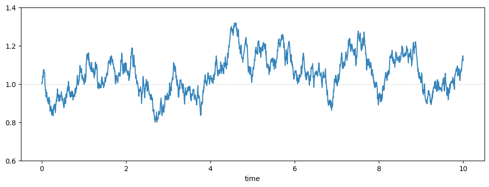
At the same time, the \(\sigma dB_t\) term constantly pushes \(X_t\) upwards and downwards in random directions. Coupled with drift, these two forces create a balance where \((X_t)\) randomly oscillates around own its mean value \(\mu \). The further away it goes, the stronger the drift term tries to bring it back. This picture is usually described as mean reversion. Here’s a sample path of \((X_t)\), with \(\mu =1\), \(\sigma =\frac 14\) and \(\theta =3\), showing random oscillations around the mean value \(1\).

More generally, for any \(X_0\in \R \) the same line of thinking shows that the OU process has a drift towards its long-term mean \(\mu \).

We can solve (13.11), at least to an extent, to obtain a useful formula for \((X_t)\). First we substitute \(Y_t=X_t-\mu \) and apply Ito’s formula to (13.11), we obtain \(dY_t=-\theta Y_t d_t+\sigma dB_t\) (this calculation is left for you). Next, set \(Z_t=e^{\theta t}Y_t\) to obtain

\begin{align*} dZ_t &= \l (\theta e^{\theta t}Y_t + e^{\theta t}(-\theta Y_t) + \frac {1}{2}(0)(\sigma )^2\r )\,dt + (e^{\theta t})(\sigma )\,dB_t \\ &=0\,dt + \sigma e^{\theta t}\,dB_t. \end{align*} In integral form we have \(Z_t-Z_0=\int _0^t \sigma e^{\theta s}\,dB_s\), and using that \(Z_t=e^{\theta t}(X_t-\mu )\) gives us

\begin{equation} \label {eq:ou_solution} X_t=\mu + e^{-\theta t}(X_0-\mu ) + \sigma \int _0^t e^{-\theta (t-s)}\,dB_s. \end{equation}

This is not quite an explicit formula, but it is still a useful representation of the OU process.

Modelling interest rates

The Ornstein-Uhlenbeck process is sometimes thought of as a model for interest rates, because of the mean reversion property. In this context it is known as the Vasicek model. We won’t discuss the reasons why interest rates display mean reversion here, save for noting that in many countries the central bank has a mandate to target a particular inflation rate (in the UK it is \(2\%\) per year). They have various tools available to try and achieve this, including increasing or decreasing the supply of money available.

The OU process is not an ideal model for interest rates, because it can take negative values whereas real interest rates essentially never become negative. For the OU process this issue may occur (even if it is very unlikely in some cases) for all choices of the model parameters. Various models have been introduced to avoid this problem, such as the Cox–Ingersoll–Ross model defined by \(dX_t=\theta (\mu -X_t)\,dt+\sigma \sqrt {X_t}\,dB_t\), for which it is known that \(\P [\text {for all }t, X_t>0]=1\) under the condition \(2\theta \mu >\sigma ^2\). We won’t be able to prove that fact within our course.