Stochastic Processes and Financial Mathematics
(part two)
\(\newcommand{\footnotename}{footnote}\)
\(\def \LWRfootnote {1}\)
\(\newcommand {\footnote }[2][\LWRfootnote ]{{}^{\mathrm {#1}}}\)
\(\newcommand {\footnotemark }[1][\LWRfootnote ]{{}^{\mathrm {#1}}}\)
\(\let \LWRorighspace \hspace \)
\(\renewcommand {\hspace }{\ifstar \LWRorighspace \LWRorighspace }\)
\(\newcommand {\mathnormal }[1]{{#1}}\)
\(\newcommand \ensuremath [1]{#1}\)
\(\newcommand {\LWRframebox }[2][]{\fbox {#2}} \newcommand {\framebox }[1][]{\LWRframebox } \)
\(\newcommand {\setlength }[2]{}\)
\(\newcommand {\addtolength }[2]{}\)
\(\newcommand {\setcounter }[2]{}\)
\(\newcommand {\addtocounter }[2]{}\)
\(\newcommand {\arabic }[1]{}\)
\(\newcommand {\number }[1]{}\)
\(\newcommand {\noalign }[1]{\text {#1}\notag \\}\)
\(\newcommand {\cline }[1]{}\)
\(\newcommand {\directlua }[1]{\text {(directlua)}}\)
\(\newcommand {\luatexdirectlua }[1]{\text {(directlua)}}\)
\(\newcommand {\protect }{}\)
\(\def \LWRabsorbnumber #1 {}\)
\(\def \LWRabsorbquotenumber "#1 {}\)
\(\newcommand {\LWRabsorboption }[1][]{}\)
\(\newcommand {\LWRabsorbtwooptions }[1][]{\LWRabsorboption }\)
\(\def \mathchar {\ifnextchar "\LWRabsorbquotenumber \LWRabsorbnumber }\)
\(\def \mathcode #1={\mathchar }\)
\(\let \delcode \mathcode \)
\(\let \delimiter \mathchar \)
\(\def \oe {\unicode {x0153}}\)
\(\def \OE {\unicode {x0152}}\)
\(\def \ae {\unicode {x00E6}}\)
\(\def \AE {\unicode {x00C6}}\)
\(\def \aa {\unicode {x00E5}}\)
\(\def \AA {\unicode {x00C5}}\)
\(\def \o {\unicode {x00F8}}\)
\(\def \O {\unicode {x00D8}}\)
\(\def \l {\unicode {x0142}}\)
\(\def \L {\unicode {x0141}}\)
\(\def \ss {\unicode {x00DF}}\)
\(\def \SS {\unicode {x1E9E}}\)
\(\def \dag {\unicode {x2020}}\)
\(\def \ddag {\unicode {x2021}}\)
\(\def \P {\unicode {x00B6}}\)
\(\def \copyright {\unicode {x00A9}}\)
\(\def \pounds {\unicode {x00A3}}\)
\(\let \LWRref \ref \)
\(\renewcommand {\ref }{\ifstar \LWRref \LWRref }\)
\( \newcommand {\multicolumn }[3]{#3}\)
\(\require {textcomp}\)
\(\newcommand {\intertext }[1]{\text {#1}\notag \\}\)
\(\let \Hat \hat \)
\(\let \Check \check \)
\(\let \Tilde \tilde \)
\(\let \Acute \acute \)
\(\let \Grave \grave \)
\(\let \Dot \dot \)
\(\let \Ddot \ddot \)
\(\let \Breve \breve \)
\(\let \Bar \bar \)
\(\let \Vec \vec \)
\( \def \offsyl {(\oslash )} \def \msconly {(\Delta )} \)
\(\DeclareMathOperator {\var }{var}\)
\(\DeclareMathOperator {\cov }{cov}\)
\(\DeclareMathOperator {\indeg }{deg_{in}}\)
\(\DeclareMathOperator {\outdeg }{deg_{out}}\)
\(\newcommand {\nN }{n \in \mathbb {N}}\)
\(\newcommand {\Br }{{\cal B}(\R )}\)
\(\newcommand {\F }{{\cal F}}\)
\(\newcommand {\ds }{\displaystyle }\)
\(\newcommand {\st }{\stackrel {d}{=}}\)
\(\newcommand {\uc }{\stackrel {uc}{\rightarrow }}\)
\(\newcommand {\la }{\langle }\)
\(\newcommand {\ra }{\rangle }\)
\(\newcommand {\li }{\liminf _{n \rightarrow \infty }}\)
\(\newcommand {\ls }{\limsup _{n \rightarrow \infty }}\)
\(\newcommand {\limn }{\lim _{n \rightarrow \infty }}\)
\(\def \ra {\Rightarrow }\)
\(\def \to {\rightarrow }\)
\(\def \iff {\Leftrightarrow }\)
\(\def \sw {\subseteq }\)
\(\def \wt {\widetilde }\)
\(\def \mc {\mathcal }\)
\(\def \mb {\mathbb }\)
\(\def \sc {\setminus }\)
\(\def \v {\textbf }\)
\(\def \p {\partial }\)
\(\def \E {\mb {E}}\)
\(\def \P {\mb {P}}\)
\(\def \R {\mb {R}}\)
\(\def \C {\mb {C}}\)
\(\def \N {\mb {N}}\)
\(\def \Q {\mb {Q}}\)
\(\def \Z {\mb {Z}}\)
\(\def \B {\mb {B}}\)
\(\def \~{\sim }\)
\(\def \-{\,;\,}\)
\(\def \|{\,|\,}\)
\(\def \qed {$\blacksquare $}\)
\(\def \1{\unicode {x1D7D9}}\)
\(\def \cadlag {c\`{a}dl\`{a}g}\)
\(\def \p {\partial }\)
\(\def \l {\left }\)
\(\def \r {\right }\)
\(\def \F {\mc {F}}\)
\(\def \G {\mc {G}}\)
\(\def \H {\mc {H}}\)
\(\def \Om {\Omega }\)
\(\def \om {\omega }\)
\(\def \Vega {\mc {V}}\)
17.3 Discontinuous stock prices and heavy tails \(\offsyl \)
We now begin to move further afield, towards some serious extensions of the standard Black-Scholes model.
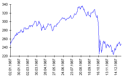
The following graph shows the Standard & Poor’s 500 index, usually known in short as the S&P 500, during 1987. It is essentially an averaged value of the stock prices of the top 500 companies within the
American stock market1. The S&P 500 is widely regarded as one of the best ways of representing, in a single number, the value of stocks within the U.S. stock markets. We won’t go into
exactly how the ‘average’ is taken.
The feature of the graph that grabs our immediate attention is the huge fall, which occurs on Monday 19th October 1987. This date has become known as Black Monday. We see an
instantaneous drop, with apparently no warning, in which the S&P 500 loses nearly 30% of its value. This is its largest fall ever, over twice the magnitude of the second largest fall (which you may remember: it
occurred on 15th October 2008).
-
Something which may strike you as very strange: no single explanation
for the Black Monday crash has ever been found. There are various theories as to what triggered the crash, ranging from a sudden lack liquidity to sudden implementations of new pricing methodology. It is often
claimed that some high-frequency trading algorithms (which were relatively new, at the time) were programmed to automatically sell stocks when they saw them drop; meaning that once a small crash
occurred there was suddenly a huge number of investors wanting to sell, exacerbating the drop in prices. However, in this case the largest drops occurred when trading volumes were low, meaning that high frequency
trading is unlikely to be the full explanation.
Of the many stock market crashes that have occurred in history, one other deserves special mention: the financial crisis of 2007-8. We will discuss it (briefly) in Chapter 18. For now, let us focus on how we might incorporate rare, but sudden, downward drops in prices into the Black-Scholes model.
A rapid downward drop in prices is best represented by a discontinuity (downwards) in the stock price. However, the theory of Ito integration that we developed only worked for continuous stochastic process. In
fact, a theory of Ito integration that can handle discontinuities does exist, but it requires much heavier use of analysis than the version we developed. The complication is that, in continuous time, we need to be clear
about what information is known instantaneously before a jump takes place – we cannot allow ourselves to foresee the jump, since this would be unrealistic. Doing so necessitates much more careful use of
\(\sigma \)-fields, filtrations and left/right-continuity than we saw in Chapter 12.
Happily, there is a generalization of Brownian motion, known as a Lévy process, which naturally incorporates unpredictable jumps, both upwards and/or downwards. It turns out that Lévy processes are
intimately connected to heavy tailed random variables (that is, where \(\E [X]\) or \(\E [X^2]\) is not defined). This, in turn, means we need a further extension of Ito calculus, to remove our reliance on \(\mc
{H}^2\) and allow for infinite means and variances. After all this theoretical work, we can then build versions of the Black-Scholes model that incorporate the possibility of rare, but unpredictable, jumps in stock
prices.
To summarize: such extensions are possible (and exist, and are used), but they are much harder to work with.