Stochastic Processes and Financial Mathematics
(part two)
\(\newcommand{\footnotename}{footnote}\)
\(\def \LWRfootnote {1}\)
\(\newcommand {\footnote }[2][\LWRfootnote ]{{}^{\mathrm {#1}}}\)
\(\newcommand {\footnotemark }[1][\LWRfootnote ]{{}^{\mathrm {#1}}}\)
\(\let \LWRorighspace \hspace \)
\(\renewcommand {\hspace }{\ifstar \LWRorighspace \LWRorighspace }\)
\(\newcommand {\mathnormal }[1]{{#1}}\)
\(\newcommand \ensuremath [1]{#1}\)
\(\newcommand {\LWRframebox }[2][]{\fbox {#2}} \newcommand {\framebox }[1][]{\LWRframebox } \)
\(\newcommand {\setlength }[2]{}\)
\(\newcommand {\addtolength }[2]{}\)
\(\newcommand {\setcounter }[2]{}\)
\(\newcommand {\addtocounter }[2]{}\)
\(\newcommand {\arabic }[1]{}\)
\(\newcommand {\number }[1]{}\)
\(\newcommand {\noalign }[1]{\text {#1}\notag \\}\)
\(\newcommand {\cline }[1]{}\)
\(\newcommand {\directlua }[1]{\text {(directlua)}}\)
\(\newcommand {\luatexdirectlua }[1]{\text {(directlua)}}\)
\(\newcommand {\protect }{}\)
\(\def \LWRabsorbnumber #1 {}\)
\(\def \LWRabsorbquotenumber "#1 {}\)
\(\newcommand {\LWRabsorboption }[1][]{}\)
\(\newcommand {\LWRabsorbtwooptions }[1][]{\LWRabsorboption }\)
\(\def \mathchar {\ifnextchar "\LWRabsorbquotenumber \LWRabsorbnumber }\)
\(\def \mathcode #1={\mathchar }\)
\(\let \delcode \mathcode \)
\(\let \delimiter \mathchar \)
\(\def \oe {\unicode {x0153}}\)
\(\def \OE {\unicode {x0152}}\)
\(\def \ae {\unicode {x00E6}}\)
\(\def \AE {\unicode {x00C6}}\)
\(\def \aa {\unicode {x00E5}}\)
\(\def \AA {\unicode {x00C5}}\)
\(\def \o {\unicode {x00F8}}\)
\(\def \O {\unicode {x00D8}}\)
\(\def \l {\unicode {x0142}}\)
\(\def \L {\unicode {x0141}}\)
\(\def \ss {\unicode {x00DF}}\)
\(\def \SS {\unicode {x1E9E}}\)
\(\def \dag {\unicode {x2020}}\)
\(\def \ddag {\unicode {x2021}}\)
\(\def \P {\unicode {x00B6}}\)
\(\def \copyright {\unicode {x00A9}}\)
\(\def \pounds {\unicode {x00A3}}\)
\(\let \LWRref \ref \)
\(\renewcommand {\ref }{\ifstar \LWRref \LWRref }\)
\( \newcommand {\multicolumn }[3]{#3}\)
\(\require {textcomp}\)
\(\newcommand {\intertext }[1]{\text {#1}\notag \\}\)
\(\let \Hat \hat \)
\(\let \Check \check \)
\(\let \Tilde \tilde \)
\(\let \Acute \acute \)
\(\let \Grave \grave \)
\(\let \Dot \dot \)
\(\let \Ddot \ddot \)
\(\let \Breve \breve \)
\(\let \Bar \bar \)
\(\let \Vec \vec \)
\( \def \offsyl {(\oslash )} \def \msconly {(\Delta )} \)
\(\DeclareMathOperator {\var }{var}\)
\(\DeclareMathOperator {\cov }{cov}\)
\(\DeclareMathOperator {\indeg }{deg_{in}}\)
\(\DeclareMathOperator {\outdeg }{deg_{out}}\)
\(\newcommand {\nN }{n \in \mathbb {N}}\)
\(\newcommand {\Br }{{\cal B}(\R )}\)
\(\newcommand {\F }{{\cal F}}\)
\(\newcommand {\ds }{\displaystyle }\)
\(\newcommand {\st }{\stackrel {d}{=}}\)
\(\newcommand {\uc }{\stackrel {uc}{\rightarrow }}\)
\(\newcommand {\la }{\langle }\)
\(\newcommand {\ra }{\rangle }\)
\(\newcommand {\li }{\liminf _{n \rightarrow \infty }}\)
\(\newcommand {\ls }{\limsup _{n \rightarrow \infty }}\)
\(\newcommand {\limn }{\lim _{n \rightarrow \infty }}\)
\(\def \ra {\Rightarrow }\)
\(\def \to {\rightarrow }\)
\(\def \iff {\Leftrightarrow }\)
\(\def \sw {\subseteq }\)
\(\def \wt {\widetilde }\)
\(\def \mc {\mathcal }\)
\(\def \mb {\mathbb }\)
\(\def \sc {\setminus }\)
\(\def \v {\textbf }\)
\(\def \p {\partial }\)
\(\def \E {\mb {E}}\)
\(\def \P {\mb {P}}\)
\(\def \R {\mb {R}}\)
\(\def \C {\mb {C}}\)
\(\def \N {\mb {N}}\)
\(\def \Q {\mb {Q}}\)
\(\def \Z {\mb {Z}}\)
\(\def \B {\mb {B}}\)
\(\def \~{\sim }\)
\(\def \-{\,;\,}\)
\(\def \|{\,|\,}\)
\(\def \qed {$\blacksquare $}\)
\(\def \1{\unicode {x1D7D9}}\)
\(\def \cadlag {c\`{a}dl\`{a}g}\)
\(\def \p {\partial }\)
\(\def \l {\left }\)
\(\def \r {\right }\)
\(\def \F {\mc {F}}\)
\(\def \G {\mc {G}}\)
\(\def \H {\mc {H}}\)
\(\def \Om {\Omega }\)
\(\def \om {\omega }\)
\(\def \Vega {\mc {V}}\)
19.5 Exercises on Chapter 19 \(\msconly \)
On random graphs and debt contagion
-
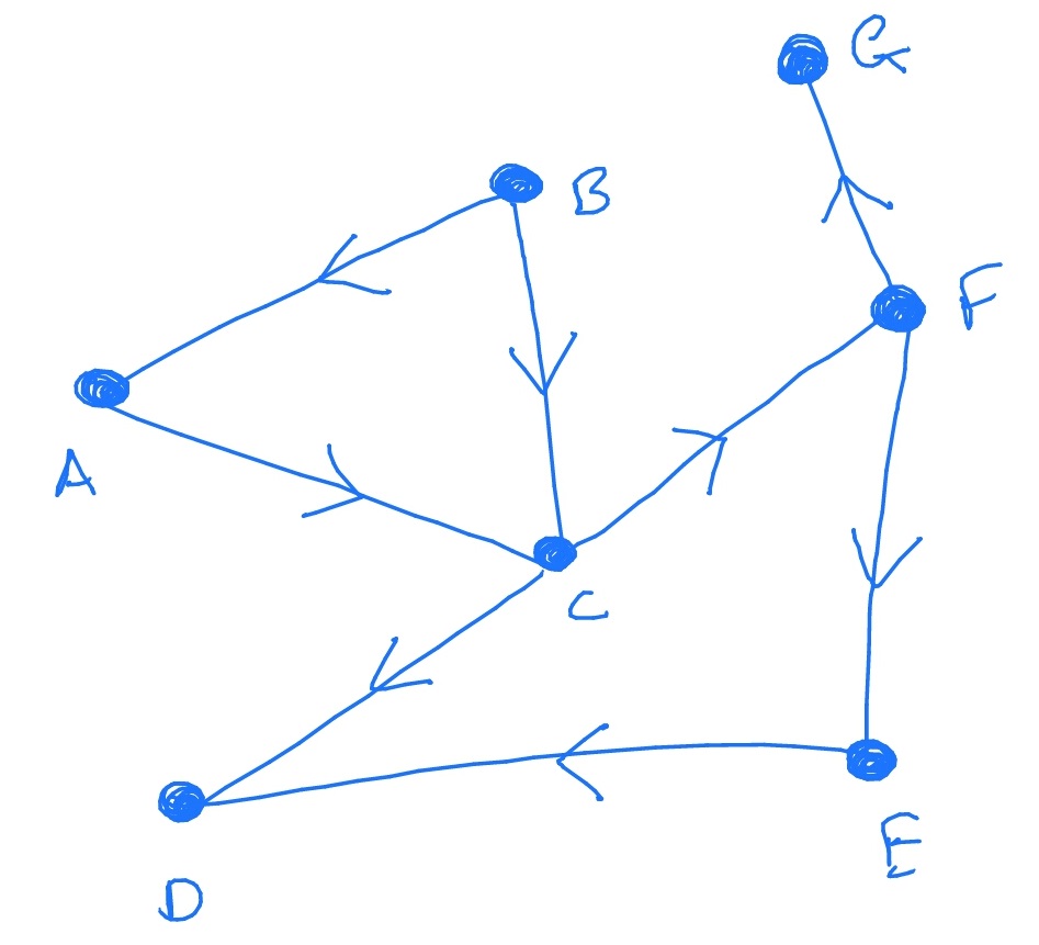
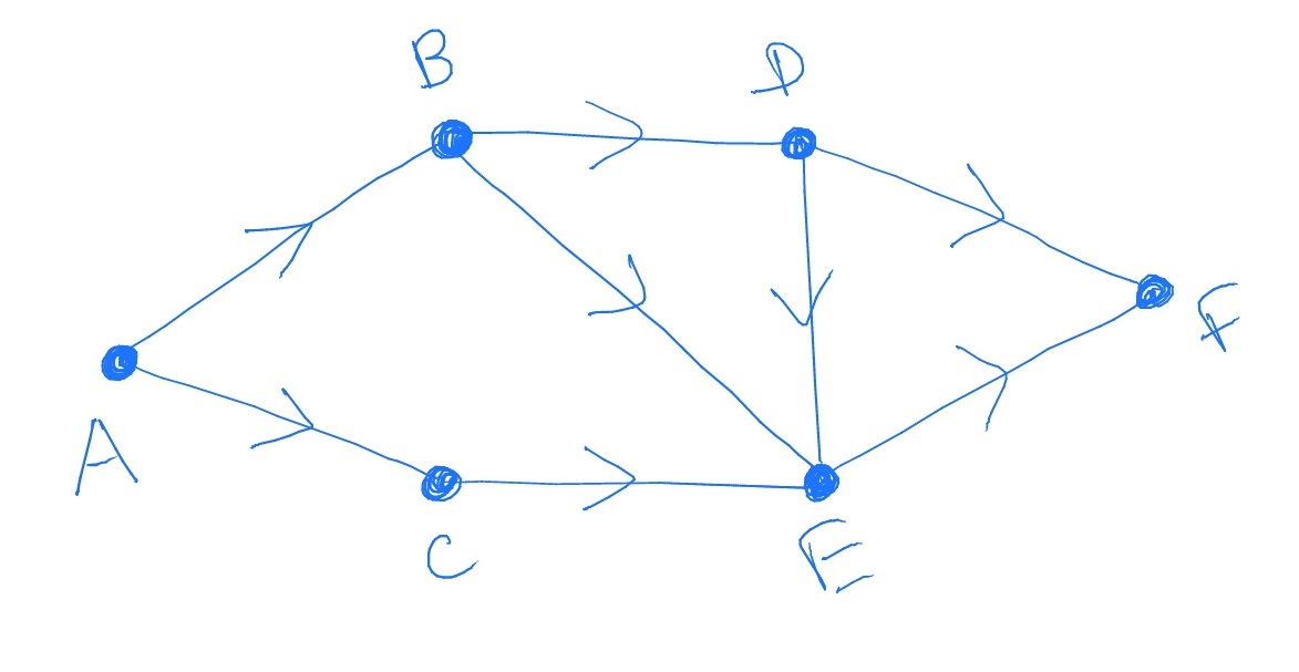
19.1 Consider the following graph \(G\). Write down the distribution of \(D_G\).
If we sample a uniformly random edge, and position ourselves at the head of this edge, what is the distribution of the out-degree \(O\) of the (random) node that we end up at?
-
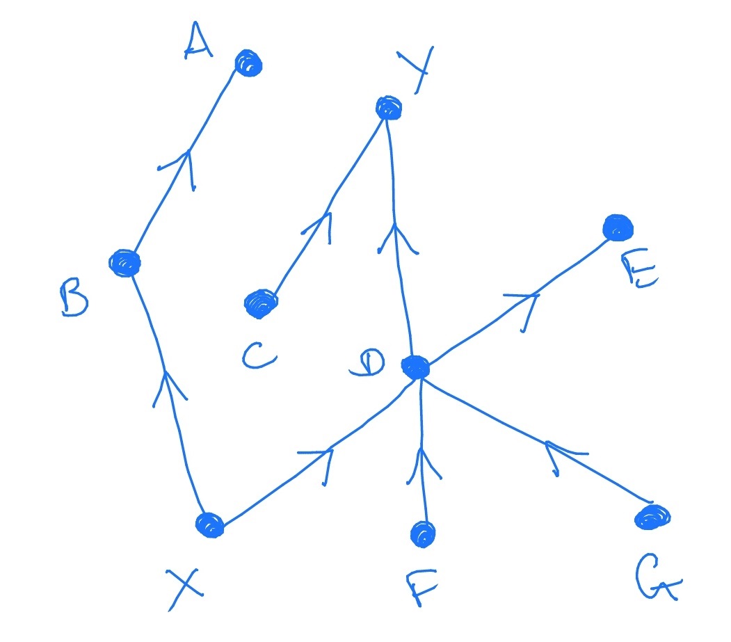
19.2 Consider the following graph, as a banking network in the Gai-Kapadia model (as described in Section 19.2).
Let the contagion probabilities be \(\eta _j=\frac 1j\). Suppose that the bank marked \(X\) fails. What is the probability that the bank marked \(Y\) also fails?
-
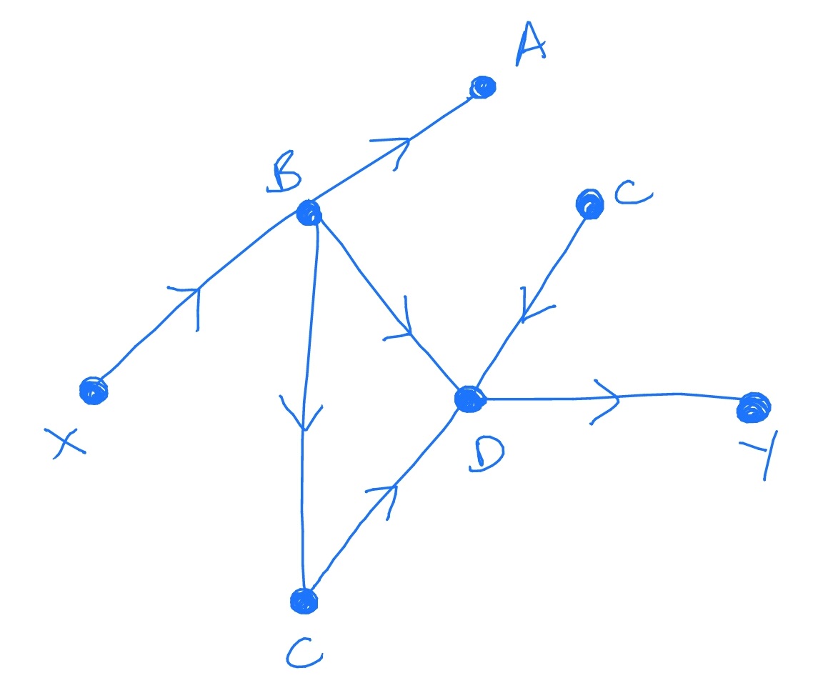
19.3 Consider the following graph, as a banking network in the Gai-Kapadia model.
Let the contagion probabilities be \(\eta _j=\frac 1j\). Suppose that the bank marked \(X\) fails. What is the probability that the bank marked \(Y\) fails?
-
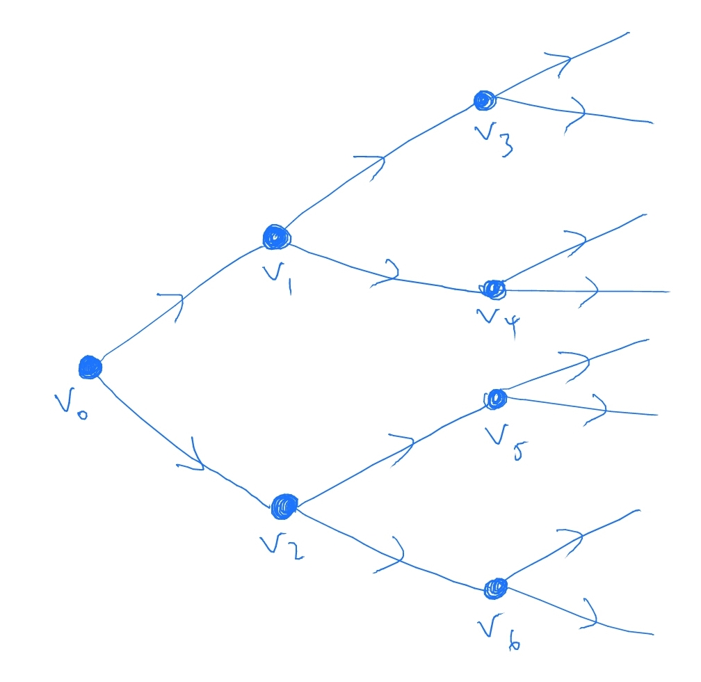
19.4 Consider the following graph (known as a binary tree) as a banking network in the Gai-Kapadia model.
This graph is a tree, with infinitely many nodes, in which every node except for \(v_0\) has one in-edge and two out-edges.
Let the contagion probabilities be \(\eta _j=\alpha \), where \(\alpha \in (0,1)\) is constant. Suppose that the bank marked \(V_0\) fails. Explain how the cascade of defaults that results can be represented
as a Galton-Watson process.
We say that a ‘catastrophic default’ occurs if an infinite number of banks fail. Under what condition on \(\alpha \) does this event have positive probability?
-
19.5 Consider the following graph, as a banking network in the Gai-Kapadia model.
Let the contagion probabilities be \(\eta _j=\frac {1}{1+j}\). Suppose that the bank marked \(A\) fails.
