Stochastic Processes and Financial Mathematics
(part two)

$\newcommand{\footnotename}{footnote}$ $\def \LWRfootnote {1}$ $\newcommand {\footnote }[2][\LWRfootnote ]{{}^{\mathrm {#1}}}$ $\newcommand {\footnotemark }[1][\LWRfootnote ]{{}^{\mathrm {#1}}}$ $\let \LWRorighspace \hspace $ $\renewcommand {\hspace }{\ifstar \LWRorighspace \LWRorighspace }$ $\newcommand {\mathnormal }[1]{{#1}}$ $\newcommand \ensuremath [1]{#1}$ $\newcommand {\LWRframebox }[2][]{\fbox {#2}} \newcommand {\framebox }[1][]{\LWRframebox } $ $\newcommand {\setlength }[2]{}$ $\newcommand {\addtolength }[2]{}$ $\newcommand {\setcounter }[2]{}$ $\newcommand {\addtocounter }[2]{}$ $\newcommand {\arabic }[1]{}$ $\newcommand {\number }[1]{}$ $\newcommand {\noalign }[1]{\text {#1}\notag \\}$ $\newcommand {\cline }[1]{}$ $\newcommand {\directlua }[1]{\text {(directlua)}}$ $\newcommand {\luatexdirectlua }[1]{\text {(directlua)}}$ $\newcommand {\protect }{}$ $\def \LWRabsorbnumber #1 {}$ $\def \LWRabsorbquotenumber "#1 {}$ $\newcommand {\LWRabsorboption }[1][]{}$ $\newcommand {\LWRabsorbtwooptions }[1][]{\LWRabsorboption }$ $\def \mathchar {\ifnextchar "\LWRabsorbquotenumber \LWRabsorbnumber }$ $\def \mathcode #1={\mathchar }$ $\let \delcode \mathcode $ $\let \delimiter \mathchar $ $\def \oe {\unicode {x0153}}$ $\def \OE {\unicode {x0152}}$ $\def \ae {\unicode {x00E6}}$ $\def \AE {\unicode {x00C6}}$ $\def \aa {\unicode {x00E5}}$ $\def \AA {\unicode {x00C5}}$ $\def \o {\unicode {x00F8}}$ $\def \O {\unicode {x00D8}}$ $\def \l {\unicode {x0142}}$ $\def \L {\unicode {x0141}}$ $\def \ss {\unicode {x00DF}}$ $\def \SS {\unicode {x1E9E}}$ $\def \dag {\unicode {x2020}}$ $\def \ddag {\unicode {x2021}}$ $\def \P {\unicode {x00B6}}$ $\def \copyright {\unicode {x00A9}}$ $\def \pounds {\unicode {x00A3}}$ $\let \LWRref \ref $ $\renewcommand {\ref }{\ifstar \LWRref \LWRref }$ $ \newcommand {\multicolumn }[3]{#3}$ $\require {textcomp}$ $\newcommand {\intertext }[1]{\text {#1}\notag \\}$ $\let \Hat \hat $ $\let \Check \check $ $\let \Tilde \tilde $ $\let \Acute \acute $ $\let \Grave \grave $ $\let \Dot \dot $ $\let \Ddot \ddot $ $\let \Breve \breve $ $\let \Bar \bar $ $\let \Vec \vec $ $\DeclareMathOperator {\var }{var}$ $\DeclareMathOperator {\cov }{cov}$ $\DeclareMathOperator {\indeg }{deg_{in}}$ $\DeclareMathOperator {\outdeg }{deg_{out}}$ $\newcommand {\nN }{n \in \mathbb {N}}$ $\newcommand {\Br }{{\cal B}(\R )}$ $\newcommand {\F }{{\cal F}}$ $\newcommand {\ds }{\displaystyle }$ $\newcommand {\st }{\stackrel {d}{=}}$ $\newcommand {\uc }{\stackrel {uc}{\rightarrow }}$ $\newcommand {\la }{\langle }$ $\newcommand {\ra }{\rangle }$ $\newcommand {\li }{\liminf _{n \rightarrow \infty }}$ $\newcommand {\ls }{\limsup _{n \rightarrow \infty }}$ $\newcommand {\limn }{\lim _{n \rightarrow \infty }}$ $\def \ra {\Rightarrow }$ $\def \to {\rightarrow }$ $\def \iff {\Leftrightarrow }$ $\def \sw {\subseteq }$ $\def \wt {\widetilde }$ $\def \mc {\mathcal }$ $\def \mb {\mathbb }$ $\def \sc {\setminus }$ $\def \v {\textbf }$ $\def \p {\partial }$ $\def \E {\mb {E}}$ $\def \P {\mb {P}}$ $\def \R {\mb {R}}$ $\def \C {\mb {C}}$ $\def \N {\mb {N}}$ $\def \Q {\mb {Q}}$ $\def \Z {\mb {Z}}$ $\def \B {\mb {B}}$ $\def \~{\sim }$ $\def \-{\,;\,}$ $\def \|{\,|\,}$ $\def \qed {$\blacksquare $}$ $\def \1{\unicode {x1D7D9}}$ $\def \cadlag {c\`{a}dl\`{a}g}$ $\def \p {\partial }$ $\def \l {\left }$ $\def \r {\right }$ $\def \F {\mc {F}}$ $\def \G {\mc {G}}$ $\def \H {\mc {H}}$ $\def \Om {\Omega }$ $\def \om {\omega }$ $\def \Vega {\mc {V}}$

19.2 The Gai-Kapadia model of debt contagion $\msconly $

Fix $n\in \N $ and take a graph $G=(V,E)$. Think of each vertex $a\in V$ as a bank, and think of each edge $(a,b)\in E$ as saying that bank $a$ has been loaned money by bank $b$.

Each loan has two possible states: healthy, or defaulted. Each bank has two possible states: healthy, or failed. Initially, all banks are assumed to be healthy, and all loans between all banks are assumed to be healthy.

We’ll make the following key assumption, that there are numbers $\eta _j\in [0,1]$ (known as contagion probabilities) such that:

$(\dagger )$ For any bank $a$, with in-degree $j$ if, at any point, $a$ is healthy and one of the loans owed to $a$ becomes defaulted, then with probability $\eta _j$ the bank $a$ fails. All loans owed by bank $a$ become defaulted.

Note that that banks who are owed a large number of loans (i.e. for which $\indeg (a)$ is large) are less likely to fail when any single one of these loans becomes defaulted. We’ll discuss how realistic this assumption is in Section 19.4.

The way the model works is as follows. To begin, a single bank is chosen uniformly at random; this bank fails and defaults on all of its loans. Because of $(\dagger )$ this (potentially) causes some other banks to default on their own loans, which in turn causes further defaults. We track the ‘cascade’ of defaults, as follows.

The set of loans which default at step $t=0,1,2,\ldots ,$ of the cascade will be denoted by $L_t$.

• On step $t=0$, we pick a single bank $a$ uniformly at random from $V=\{1,\ldots ,n\}$. This banks fails, and all defaults on all of its loans: we set $D_0$ to be the set of out-edges of $a$.
• Then, iteratively, for $t=1,2,\ldots $, we construct $L_t$ as follows.

For each $(b,c)\in L_{t-1}$, we apply $(\dagger )$ to $c$. That is, if $c$ is healthy then $c$ fails with probability $\eta _{\indeg (c)}$. If this causes $c$ to fail, then we include all out-edges of $c$ into $L_t$.

Eventually, because there are only finitely many edges in the graph, we reach a point at which $L_t$ is empty. From then on, $L_{t+1},L_{t+2}$ are also empty. Then, the set of loans which were defaulted on during the cascade is

\begin{equation} \label {eq:L_cascade} \mathscr {L}=\bigcup \limits _{i=1}^\infty L_t. \end{equation}

We’ll be interested in working out how big the set $\mathscr {L}$ is. That is, we are interested to know how many loans become defaulted once cascade finishes.

Remark 19.2.1 In reality, the main object of interest is how many banks fail during the cascade. This is closely connected to how many loans default but, for simplicity, we choose to focus on loans.

A summary of this model appears on the formula sheet, see Appendix E. We refer to it as the Gai-Kapadia model (of debt contagion). The parameters $\eta _j$ are known as the contagion probabilities.

We’ll now look at an example of the steps the cascade could take, on the graph we used as an example in Section 19.1. We’ll mark defaulted/failed edges/nodes as red and take $\eta _j=\frac 1j$. Initially, let us say that node $B$ fails and defaults on the loan it owes to $C$:

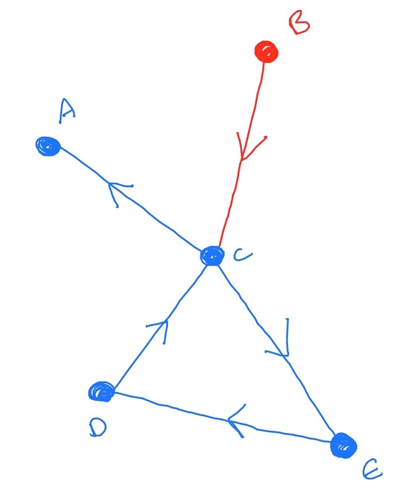
Since $C$ has two in-edges, and $\eta _2=\frac 12$, $C$ has a probability $\frac 12$ of failing as a result of this default. So - we toss a coin and lets say that we discover that $C$ does fail. Then $C$ also defaults on all its loans:

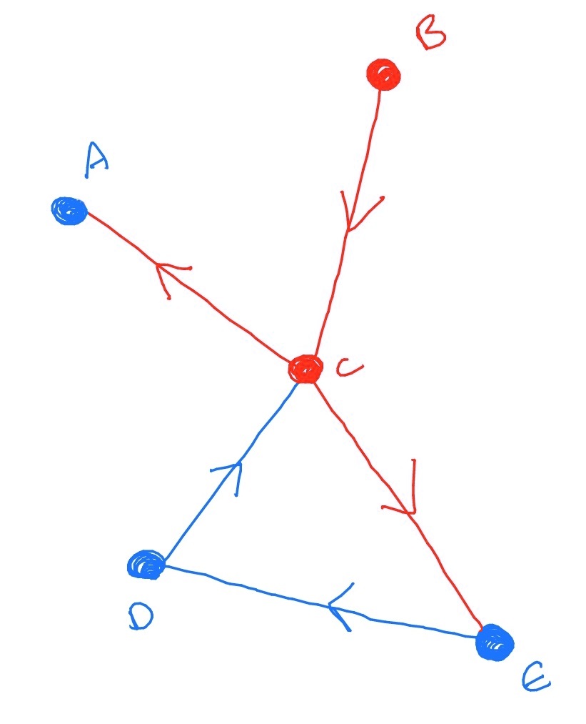
Now, both $E$ and $A$ have only a single in-edge. Since $\eta _1=1$ this makes them certain to fail when their single debtor defaults. Similarly, $D$ also fails. So the final result is that the whole graph is defaulted.

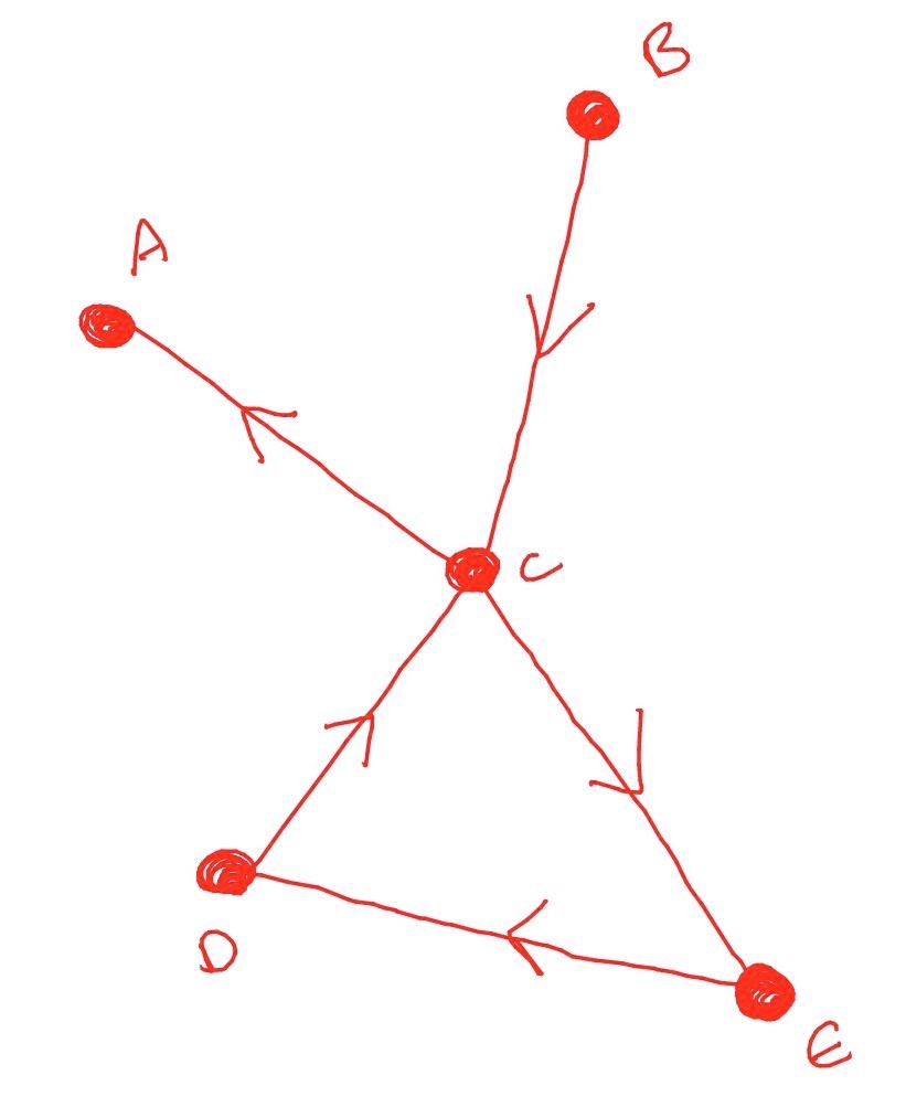
Of course, it didn’t have to be this way. If our coin toss had gone the other way and $C$ had not failed, the cascade would have finished after its first step and the final graph would simply look like

So we obtain that these two outcomes are both possible, each with probability $\frac 12$. Of course, in a bigger graph, the range of possible outcomes can be very large.

Stochastic Processes and Financial Mathematics (part two)

19.2 The Gai-Kapadia model of debt contagion \(\msconly \)

Stochastic Processes and Financial Mathematics
(part two)