Bayesian Statistics

$\newcommand{\footnotename}{footnote}$ $\def \LWRfootnote {1}$ $\newcommand {\footnote }[2][\LWRfootnote ]{{}^{\mathrm {#1}}}$ $\newcommand {\footnotemark }[1][\LWRfootnote ]{{}^{\mathrm {#1}}}$ $\let \LWRorighspace \hspace $ $\renewcommand {\hspace }{\ifstar \LWRorighspace \LWRorighspace }$ $\newcommand {\mathnormal }[1]{{#1}}$ $\newcommand \ensuremath [1]{#1}$ $\newcommand {\LWRframebox }[2][]{\fbox {#2}} \newcommand {\framebox }[1][]{\LWRframebox } $ $\newcommand {\setlength }[2]{}$ $\newcommand {\addtolength }[2]{}$ $\newcommand {\setcounter }[2]{}$ $\newcommand {\addtocounter }[2]{}$ $\newcommand {\arabic }[1]{}$ $\newcommand {\number }[1]{}$ $\newcommand {\noalign }[1]{\text {#1}\notag \\}$ $\newcommand {\cline }[1]{}$ $\newcommand {\directlua }[1]{\text {(directlua)}}$ $\newcommand {\luatexdirectlua }[1]{\text {(directlua)}}$ $\newcommand {\protect }{}$ $\def \LWRabsorbnumber #1 {}$ $\def \LWRabsorbquotenumber "#1 {}$ $\newcommand {\LWRabsorboption }[1][]{}$ $\newcommand {\LWRabsorbtwooptions }[1][]{\LWRabsorboption }$ $\def \mathchar {\ifnextchar "\LWRabsorbquotenumber \LWRabsorbnumber }$ $\def \mathcode #1={\mathchar }$ $\let \delcode \mathcode $ $\let \delimiter \mathchar $ $\def \oe {\unicode {x0153}}$ $\def \OE {\unicode {x0152}}$ $\def \ae {\unicode {x00E6}}$ $\def \AE {\unicode {x00C6}}$ $\def \aa {\unicode {x00E5}}$ $\def \AA {\unicode {x00C5}}$ $\def \o {\unicode {x00F8}}$ $\def \O {\unicode {x00D8}}$ $\def \l {\unicode {x0142}}$ $\def \L {\unicode {x0141}}$ $\def \ss {\unicode {x00DF}}$ $\def \SS {\unicode {x1E9E}}$ $\def \dag {\unicode {x2020}}$ $\def \ddag {\unicode {x2021}}$ $\def \P {\unicode {x00B6}}$ $\def \copyright {\unicode {x00A9}}$ $\def \pounds {\unicode {x00A3}}$ $\let \LWRref \ref $ $\renewcommand {\ref }{\ifstar \LWRref \LWRref }$ $ \newcommand {\multicolumn }[3]{#3}$ $\require {textcomp}$ $\newcommand {\intertext }[1]{\text {#1}\notag \\}$ $\let \Hat \hat $ $\let \Check \check $ $\let \Tilde \tilde $ $\let \Acute \acute $ $\let \Grave \grave $ $\let \Dot \dot $ $\let \Ddot \ddot $ $\let \Breve \breve $ $\let \Bar \bar $ $\let \Vec \vec $ $\require {colortbl}$ $\let \LWRorigcolumncolor \columncolor $ $\renewcommand {\columncolor }[2][named]{\LWRorigcolumncolor [#1]{#2}\LWRabsorbtwooptions }$ $\let \LWRorigrowcolor \rowcolor $ $\renewcommand {\rowcolor }[2][named]{\LWRorigrowcolor [#1]{#2}\LWRabsorbtwooptions }$ $\let \LWRorigcellcolor \cellcolor $ $\renewcommand {\cellcolor }[2][named]{\LWRorigcellcolor [#1]{#2}\LWRabsorbtwooptions }$ $\require {mathtools}$ $\newenvironment {crampedsubarray}[1]{}{}$ $\newcommand {\smashoperator }[2][]{#2\limits }$ $\newcommand {\SwapAboveDisplaySkip }{}$ $\newcommand {\LaTeXunderbrace }[1]{\underbrace {#1}}$ $\newcommand {\LaTeXoverbrace }[1]{\overbrace {#1}}$ $\newcommand {\LWRmultlined }[1][]{\begin {multline*}}$ $\newenvironment {multlined}[1][]{\LWRmultlined }{\end {multline*}}$ $\let \LWRorigshoveleft \shoveleft $ $\renewcommand {\shoveleft }[1][]{\LWRorigshoveleft }$ $\let \LWRorigshoveright \shoveright $ $\renewcommand {\shoveright }[1][]{\LWRorigshoveright }$ $\newcommand {\shortintertext }[1]{\text {#1}\notag \\}$ $\newcommand {\vcentcolon }{\mathrel {\unicode {x2236}}}$ $\renewcommand {\intertext }[2][]{\text {#2}\notag \\}$ $\newenvironment {fleqn}[1][]{}{}$ $\newenvironment {ceqn}{}{}$ $\newenvironment {darray}[2][c]{\begin {array}[#1]{#2}}{\end {array}}$ $\newcommand {\dmulticolumn }[3]{#3}$ $\newcommand {\LWRnrnostar }[1][0.5ex]{\\[#1]}$ $\newcommand {\nr }{\ifstar \LWRnrnostar \LWRnrnostar }$ $\newcommand {\mrel }[1]{\begin {aligned}#1\end {aligned}}$ $\newcommand {\underrel }[2]{\underset {#2}{#1}}$ $\newcommand {\medmath }[1]{#1}$ $\newcommand {\medop }[1]{#1}$ $\newcommand {\medint }[1]{#1}$ $\newcommand {\medintcorr }[1]{#1}$ $\newcommand {\mfrac }[2]{\frac {#1}{#2}}$ $\newcommand {\mbinom }[2]{\binom {#1}{#2}}$ $\newenvironment {mmatrix}{\begin {matrix}}{\end {matrix}}$ $\newcommand {\displaybreak }[1][]{}$ $ \def \offsyl {(\oslash )} \def \msconly {(\Delta )} $ $ \DeclareMathOperator {\var }{var} \DeclareMathOperator {\cov }{cov} \DeclareMathOperator {\Bin }{Bin} \DeclareMathOperator {\Geo }{Geometric} \DeclareMathOperator {\Beta }{Beta} \DeclareMathOperator {\Unif }{Uniform} \DeclareMathOperator {\Gam }{Gamma} \DeclareMathOperator {\Normal }{N} \DeclareMathOperator {\Exp }{Exp} \DeclareMathOperator {\Cauchy }{Cauchy} \DeclareMathOperator {\Bern }{Bernoulli} \DeclareMathOperator {\Poisson }{Poisson} \DeclareMathOperator {\Weibull }{Weibull} \DeclareMathOperator {\IGam }{IGamma} \DeclareMathOperator {\NGam }{NGamma} \DeclareMathOperator {\ChiSquared }{ChiSquared} \DeclareMathOperator {\Pareto }{Pareto} \DeclareMathOperator {\NBin }{NegBin} \DeclareMathOperator {\Studentt }{Student-t} \DeclareMathOperator *{\argmax }{arg\,max} \DeclareMathOperator *{\argmin }{arg\,min} $ \( \def \to {\rightarrow } \def \iff {\Leftrightarrow } \def \ra {\Rightarrow } \def \sw {\subseteq } \def \mc {\mathcal } \def \mb {\mathbb } \def \sc {\setminus } \def \wt {\widetilde } \def \v {\textbf } \def \E {\mb {E}} \def \P {\mb {P}} \def \R {\mb {R}} \def \C {\mb {C}} \def \N {\mb {N}} \def \Q {\mb {Q}} \def \Z {\mb {Z}} \def \B {\mb {B}} \def \~{\sim } \def \-{\,;\,} \def \qed {$\blacksquare $} \CustomizeMathJax {\def \1{\unicode {x1D7D9}}} \def \cadlag {c\`{a}dl\`{a}g} \def \p {\partial } \def \l {\left } \def \r {\right } \def \Om {\Omega } \def \om {\omega } \def \eps {\epsilon } \def \de {\delta } \def \ov {\overline } \def \sr {\stackrel } \def \Lp {\mc {L}^p} \def \Lq {\mc {L}^p} \def \Lone {\mc {L}^1} \def \Ltwo {\mc {L}^2} \def \toae {\sr {\rm a.e.}{\to }} \def \toas {\sr {\rm a.s.}{\to }} \def \top {\sr {\mb {\P }}{\to }} \def \tod {\sr {\rm d}{\to }} \def \toLp {\sr {\Lp }{\to }} \def \toLq {\sr {\Lq }{\to }} \def \eqae {\sr {\rm a.e.}{=}} \def \eqas {\sr {\rm a.s.}{=}} \def \eqd {\sr {\rm d}{=}} \def \approxd {\sr {\rm d}{\approx }} \def \Sa {(S1)\xspace } \def \Sb {(S2)\xspace } \def \Sc {(S3)\xspace } \)

1.6 Conditioning on events with zero probability

Lemma 1.4.1 requires that the event $A$, on which we condition, has positive probability. Without that condition equation (1.4) would become $\frac {0}{0}$, which is undefined. Despite this problem it is often possible to make sense of the result of conditioning on an event of probability zero. The mathematical theory here is much more complicated than we can cover, so instead we will explain the key idea and focus on a small set of well-behaved situations.

We will take a random variable $(Y,Z)$ and condition $Z$ on the event $\{Y=y\}$, where $Y$ is continuous. In this case $\P [Y=y]=0$. The key idea is this: if there exists a random variable $Z^*$ such that

\begin{equation} \label {eq:conditioning_eps_to_0} \P \l [Z|_{\{|Y-y|\leq \eps \}}\in A\r ]\to \P [Z^*\in A] \qquad \text { as }\eps \to 0 \end{equation}

for all $A\sw \R ^n$, then we extend Definition 1.4.2; we say that $Z^*$ is the conditional distribution of $Z$ given $\{Y=y\}$, written $Z^*\eqd Z|_{\{Y=y\}}$. There are many examples of random variables $(Y,Z)$ for which the limit in (1.9) does not exist, or fails to behave like a conditional probability. There are, also, many examples where (1.9) results in a random variable $Y$ that behaves exactly like we would expect, based on the intuition we have built up from Lemma 1.4.1.

Here is a case where it does work, that you’ve seen before. In earlier courses you may have been told that (1.10) was the definition of a conditional p.d.f., but that is not entirely honest. It is a consequence of (1.9) and it requires some conditions.

Lemma 1.6.1 Let $(Y,Z)$ be continuous random variables, where $Y$ takes values in $\R ^n$ and $Z$ takes values in $\R ^d$. Suppose that $f_Y(y)>0$ and that both $f_Y(y)$ and $f_{Y,Z}(y,z)$ are continuous functions. Then $Z|_{\{Y=y\}}$ is a continuous random variable with p.d.f.
$\seteqnumber{0}{1.}{9}$
\begin{equation} \label {eq:conditional_pdf} f_{Z|_{\{Y=y\}}}(z)=\frac {f_{Y,Z}(y,z)}{f_Y(y)}. \end{equation}

Proof: $\offsyl $ We will sketch an argument to show why the result holds, but we won’t include a proof here. For simplicity, let us assume that $Y$ and $Z$ both takes values in $\R $. From Lemma 1.5.1 we have

\begin{align*} \P [Z|_{\{|Y-y|\leq \eps \}}\in B] =\frac {\P [|Y-y|\leq \eps , Z\in B]}{\P [|Y-y|\leq \eps ]} =\frac {\int _B\int _{y-\eps }^{y+\eps } f_{Y,Z}(u,z)\,du\,dz}{\int _{y-\eps }^{y+\eps }f_Y(u)\,du}. \end{align*} Our continuity assumptions mean that when $\eps $ is small and $|u-y|\leq \eps $, we can approximate $f_{Y,Z}(u,z)\approx f_{Y,Z}(y,z)$ and $f_Y(u)\approx f_Y(y)$. Putting both these approximations in,

\begin{align} \P [Z|_{\{|Y-y|\leq \eps \}}\in B] \approx \frac {\int _B\int _{y-\eps }^{y+\eps } f_{Y,Z}(y,z)\,du\,dz}{\int _{y-\eps }^{y+\eps }f_Y(u)\,du} =\frac {2\eps \int _B f_{Y,Z}(y,z)\,dz}{2\eps f_Y(y)} =\int _B \frac {f_{Y,Z}(y,z)}{f_Y(y)}\,dz. \label {eq:cond_pdf_proof} \end{align} Because of our approximation the right hand side of (1.11) does not contain $\eps $. This suggests that letting $\eps \to 0$ should result in $\lim _{\eps \to 0} \P [Z|_{\{|Y-y|\leq \eps \}}\in B]=\int _B \frac {f_{Y,Z}(y,z)}{f_Y(y)}\,dz$. Combining this formula with Definition 1.1.1 and (1.9) gives that $Z|_{\{Y=y\}}$ exists and is a continuous random variable, with the p.d.f. as claimed. ∎

Example 1.6.2 Let $(Y,Z)$ be a continuous random variable taking values in $\R ^2$, with (joint) probability density function
$\seteqnumber{0}{1.}{11}$
\begin{equation} \label {eq:pdf_family_ex} f_{(Y,Z)}(y,z)= \frac {1}{\sqrt {2\pi ^3}}\frac {e^{-y^2/2}}{1+(z-y)^2}. \end{equation}

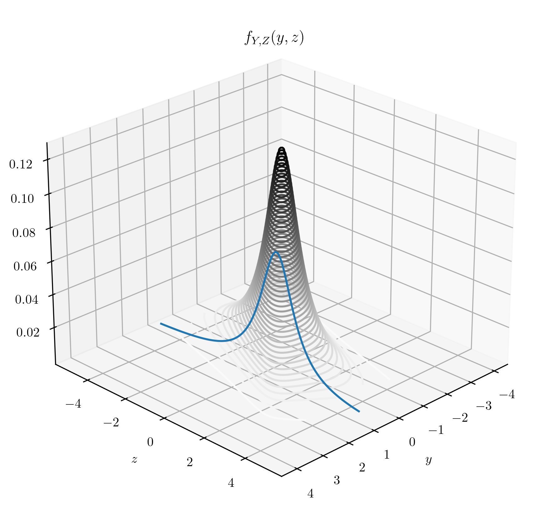
for all $y,z\in \R $. Note that this is a continuous function (or see the plot below). We can compute
$\seteqnumber{0}{1.}{12}$
\begin{align*} f_Y(y) =\int _\R f_{Y,Z}(y,z)\,dz &=\frac {1}{\sqrt {2\pi ^3}}e^{-y^2/2}\int _{-\infty }^\infty \frac {1}{1+(z-y)^2}\,dz \\ &=\frac {1}{\sqrt {2\pi ^3}}e^{-y^2/2}\int _{-\infty }^\infty \frac {1}{1+z^2}\,dz \\ &=\frac {1}{\sqrt {2\pi ^3}}e^{-y^2/2}[\arctan (z)]_{-\infty }^\infty \\ &=\frac {1}{\sqrt {2\pi ^3}}e^{-y^2/2}\l (\frac {\pi }{2}-\frac {-\pi }{2}\r ) \\ &=\frac {1}{\sqrt {2\pi }}e^{-y^2/2}, \end{align*} 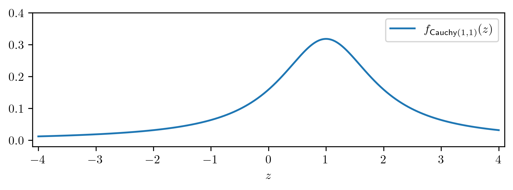which we recognize as $Y\sim \Normal (0,1)$. We will condition on $\{Y=1\}$. Clearly $f_Y(1)>0$, so Lemma 1.6.1 applies, and we obtain
$\seteqnumber{0}{1.}{12}$
\begin{equation*} f_{Z|_{\{Y=1\}}}(y) =\frac {f_{Y,Z}(1,z)}{f_Y(1)} =\frac {\frac {1}{\sqrt {2\pi ^3}}\frac {e^{-1}}{1+(z-1)^2}}{\frac {1}{\sqrt {2\pi }}e^{-1}} =\frac {1}{\pi }\frac {1}{1+(z-1)^2} \end{equation*}

which we recognize as $Z|_{\{Y=1\}}\sim \Cauchy (1,1)$. We can plot $f_{Y,Z}(y,z)$ and $f_{Z|_{\{Y=1\}}}$ as follows:

The line on the left hand picture corresponds to $y=1$. You can see that it has the shape of the $\Cauchy (1,1)$ p.d.f. in the right hand picture.

Remark 1.6.3 $\offsyl $ It is possible to extend Lemma 1.6.1 to weaken the assumption of continuity. This requires some care and we won’t explore the details here, although we will sometimes use (1.10) in these cases. As a general rule it is dangerous to condition when $f_{Y,Z}(y,z)$ features discontinuities that might influence the conditioning.

Remark 1.6.4 Taking $Y=Z$ in (1.9), a similar approximation argument to the proof of Lemma 1.6.1 shows that for a continuous random variable $Y$ and $y\in \R _Y$, we have $Y|_{\{Y=y\}}\eqd y$. We already knew this for discrete random variables, in Lemma 1.4.4, so it is hopefully easy to believe. We record this fact because we will need it in Chapter 8.