Bayesian Statistics

$\newcommand{\footnotename}{footnote}$ $\def \LWRfootnote {1}$ $\newcommand {\footnote }[2][\LWRfootnote ]{{}^{\mathrm {#1}}}$ $\newcommand {\footnotemark }[1][\LWRfootnote ]{{}^{\mathrm {#1}}}$ $\let \LWRorighspace \hspace $ $\renewcommand {\hspace }{\ifstar \LWRorighspace \LWRorighspace }$ $\newcommand {\mathnormal }[1]{{#1}}$ $\newcommand \ensuremath [1]{#1}$ $\newcommand {\LWRframebox }[2][]{\fbox {#2}} \newcommand {\framebox }[1][]{\LWRframebox } $ $\newcommand {\setlength }[2]{}$ $\newcommand {\addtolength }[2]{}$ $\newcommand {\setcounter }[2]{}$ $\newcommand {\addtocounter }[2]{}$ $\newcommand {\arabic }[1]{}$ $\newcommand {\number }[1]{}$ $\newcommand {\noalign }[1]{\text {#1}\notag \\}$ $\newcommand {\cline }[1]{}$ $\newcommand {\directlua }[1]{\text {(directlua)}}$ $\newcommand {\luatexdirectlua }[1]{\text {(directlua)}}$ $\newcommand {\protect }{}$ $\def \LWRabsorbnumber #1 {}$ $\def \LWRabsorbquotenumber "#1 {}$ $\newcommand {\LWRabsorboption }[1][]{}$ $\newcommand {\LWRabsorbtwooptions }[1][]{\LWRabsorboption }$ $\def \mathchar {\ifnextchar "\LWRabsorbquotenumber \LWRabsorbnumber }$ $\def \mathcode #1={\mathchar }$ $\let \delcode \mathcode $ $\let \delimiter \mathchar $ $\def \oe {\unicode {x0153}}$ $\def \OE {\unicode {x0152}}$ $\def \ae {\unicode {x00E6}}$ $\def \AE {\unicode {x00C6}}$ $\def \aa {\unicode {x00E5}}$ $\def \AA {\unicode {x00C5}}$ $\def \o {\unicode {x00F8}}$ $\def \O {\unicode {x00D8}}$ $\def \l {\unicode {x0142}}$ $\def \L {\unicode {x0141}}$ $\def \ss {\unicode {x00DF}}$ $\def \SS {\unicode {x1E9E}}$ $\def \dag {\unicode {x2020}}$ $\def \ddag {\unicode {x2021}}$ $\def \P {\unicode {x00B6}}$ $\def \copyright {\unicode {x00A9}}$ $\def \pounds {\unicode {x00A3}}$ $\let \LWRref \ref $ $\renewcommand {\ref }{\ifstar \LWRref \LWRref }$ $ \newcommand {\multicolumn }[3]{#3}$ $\require {textcomp}$ $\newcommand {\intertext }[1]{\text {#1}\notag \\}$ $\let \Hat \hat $ $\let \Check \check $ $\let \Tilde \tilde $ $\let \Acute \acute $ $\let \Grave \grave $ $\let \Dot \dot $ $\let \Ddot \ddot $ $\let \Breve \breve $ $\let \Bar \bar $ $\let \Vec \vec $ $\require {colortbl}$ $\let \LWRorigcolumncolor \columncolor $ $\renewcommand {\columncolor }[2][named]{\LWRorigcolumncolor [#1]{#2}\LWRabsorbtwooptions }$ $\let \LWRorigrowcolor \rowcolor $ $\renewcommand {\rowcolor }[2][named]{\LWRorigrowcolor [#1]{#2}\LWRabsorbtwooptions }$ $\let \LWRorigcellcolor \cellcolor $ $\renewcommand {\cellcolor }[2][named]{\LWRorigcellcolor [#1]{#2}\LWRabsorbtwooptions }$ $\require {mathtools}$ $\newenvironment {crampedsubarray}[1]{}{}$ $\newcommand {\smashoperator }[2][]{#2\limits }$ $\newcommand {\SwapAboveDisplaySkip }{}$ $\newcommand {\LaTeXunderbrace }[1]{\underbrace {#1}}$ $\newcommand {\LaTeXoverbrace }[1]{\overbrace {#1}}$ $\newcommand {\LWRmultlined }[1][]{\begin {multline*}}$ $\newenvironment {multlined}[1][]{\LWRmultlined }{\end {multline*}}$ $\let \LWRorigshoveleft \shoveleft $ $\renewcommand {\shoveleft }[1][]{\LWRorigshoveleft }$ $\let \LWRorigshoveright \shoveright $ $\renewcommand {\shoveright }[1][]{\LWRorigshoveright }$ $\newcommand {\shortintertext }[1]{\text {#1}\notag \\}$ $\newcommand {\vcentcolon }{\mathrel {\unicode {x2236}}}$ $\renewcommand {\intertext }[2][]{\text {#2}\notag \\}$ $\newenvironment {fleqn}[1][]{}{}$ $\newenvironment {ceqn}{}{}$ $\newenvironment {darray}[2][c]{\begin {array}[#1]{#2}}{\end {array}}$ $\newcommand {\dmulticolumn }[3]{#3}$ $\newcommand {\LWRnrnostar }[1][0.5ex]{\\[#1]}$ $\newcommand {\nr }{\ifstar \LWRnrnostar \LWRnrnostar }$ $\newcommand {\mrel }[1]{\begin {aligned}#1\end {aligned}}$ $\newcommand {\underrel }[2]{\underset {#2}{#1}}$ $\newcommand {\medmath }[1]{#1}$ $\newcommand {\medop }[1]{#1}$ $\newcommand {\medint }[1]{#1}$ $\newcommand {\medintcorr }[1]{#1}$ $\newcommand {\mfrac }[2]{\frac {#1}{#2}}$ $\newcommand {\mbinom }[2]{\binom {#1}{#2}}$ $\newenvironment {mmatrix}{\begin {matrix}}{\end {matrix}}$ $\newcommand {\displaybreak }[1][]{}$ $ \def \offsyl {(\oslash )} \def \msconly {(\Delta )} $ $ \DeclareMathOperator {\var }{var} \DeclareMathOperator {\cov }{cov} \DeclareMathOperator {\Bin }{Bin} \DeclareMathOperator {\Geo }{Geometric} \DeclareMathOperator {\Beta }{Beta} \DeclareMathOperator {\Unif }{Uniform} \DeclareMathOperator {\Gam }{Gamma} \DeclareMathOperator {\Normal }{N} \DeclareMathOperator {\Exp }{Exp} \DeclareMathOperator {\Cauchy }{Cauchy} \DeclareMathOperator {\Bern }{Bernoulli} \DeclareMathOperator {\Poisson }{Poisson} \DeclareMathOperator {\Weibull }{Weibull} \DeclareMathOperator {\IGam }{IGamma} \DeclareMathOperator {\NGam }{NGamma} \DeclareMathOperator {\ChiSquared }{ChiSquared} \DeclareMathOperator {\Pareto }{Pareto} \DeclareMathOperator {\NBin }{NegBin} \DeclareMathOperator {\Studentt }{Student-t} \DeclareMathOperator *{\argmax }{arg\,max} \DeclareMathOperator *{\argmin }{arg\,min} $ \( \def \to {\rightarrow } \def \iff {\Leftrightarrow } \def \ra {\Rightarrow } \def \sw {\subseteq } \def \mc {\mathcal } \def \mb {\mathbb } \def \sc {\setminus } \def \wt {\widetilde } \def \v {\textbf } \def \E {\mb {E}} \def \P {\mb {P}} \def \R {\mb {R}} \def \C {\mb {C}} \def \N {\mb {N}} \def \Q {\mb {Q}} \def \Z {\mb {Z}} \def \B {\mb {B}} \def \~{\sim } \def \-{\,;\,} \def \qed {$\blacksquare $} \CustomizeMathJax {\def \1{\unicode {x1D7D9}}} \def \cadlag {c\`{a}dl\`{a}g} \def \p {\partial } \def \l {\left } \def \r {\right } \def \Om {\Omega } \def \om {\omega } \def \eps {\epsilon } \def \de {\delta } \def \ov {\overline } \def \sr {\stackrel } \def \Lp {\mc {L}^p} \def \Lq {\mc {L}^p} \def \Lone {\mc {L}^1} \def \Ltwo {\mc {L}^2} \def \toae {\sr {\rm a.e.}{\to }} \def \toas {\sr {\rm a.s.}{\to }} \def \top {\sr {\mb {\P }}{\to }} \def \tod {\sr {\rm d}{\to }} \def \toLp {\sr {\Lp }{\to }} \def \toLq {\sr {\Lq }{\to }} \def \eqae {\sr {\rm a.e.}{=}} \def \eqas {\sr {\rm a.s.}{=}} \def \eqd {\sr {\rm d}{=}} \def \approxd {\sr {\rm d}{\approx }} \def \Sa {(S1)\xspace } \def \Sb {(S2)\xspace } \def \Sc {(S3)\xspace } \)

4.4 What if?

In this section we do some numerical experiments to illustrate the sort of things that go wrong if, for some reason, our model family or our prior is too unrealistic. We will first describe a situation where the inference works as intended, and then we’ll do some things to break it.

Example 4.4.1 Let $(X,\Theta )$ be a continuous Bayesian model with model family $M_\lambda \sim \Exp (\lambda )^{\otimes n}$ and parameter $\lambda \in (0,\infty )$. Take the prior to be $\Theta \sim \Gamma (\alpha ,\beta )$, where $\alpha ,\beta \in (0,\infty )$.

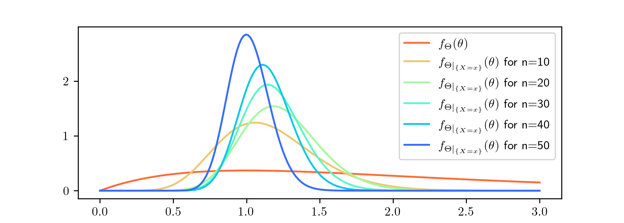
For now, we choose the prior with $\alpha =\beta =1$. We will feed our model data consisting of i.i.d. samples from the $\Exp (1)$ distribution. This corresponds to a true value of the parameter given by $\lambda ^*=1$. In other words, if we set $\Theta =\lambda $ in our Bayesian model then the samples it would produce for $X$ would have exactly the same distribution as the data. So, we hope that Bayesian updates based on this data will result in a posterior density with its mass near to $1$.

The posterior densities that resulted from various amounts of data $x$, sampled from $\Exp (1)^{\otimes n}$, are as follows.

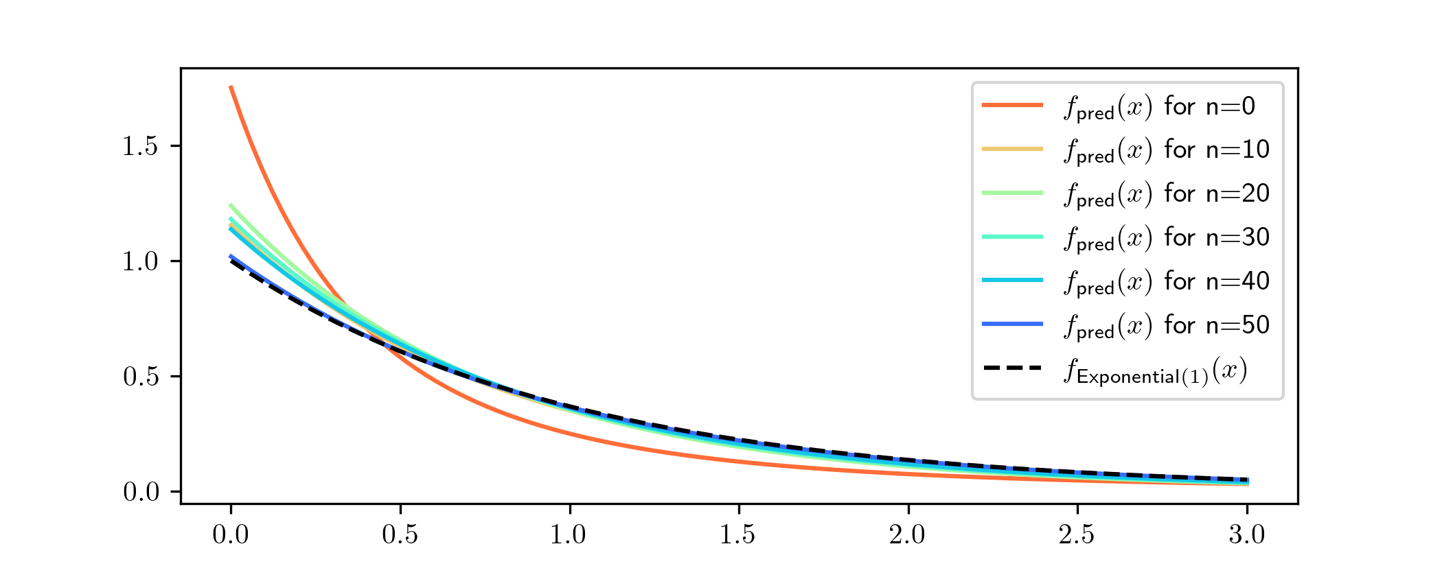
The Bayesian updates here were calculated using Lemma 4.2.1. As expected, although the mass of our prior is not close to the true value, we can see the posterior densities becoming more and more focused on the value $1$. We can also see the corresponding predictive distributions (for a single datapoint) converging towards $\Exp (1)$. The density functions look like:

What if the model is wrong?

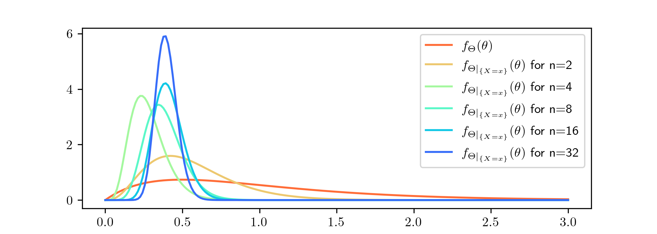
Example 4.4.2 Here we use the same model as in Example 4.4.1, but now we feed our model data consisting of i.i.d. samples from the $\ChiSquared (2)$ distribution. In this case there is no value of the parameter $\lambda $ for which our model $(X,\Theta )$ is a good representation of the data. We are interested to see what happens:

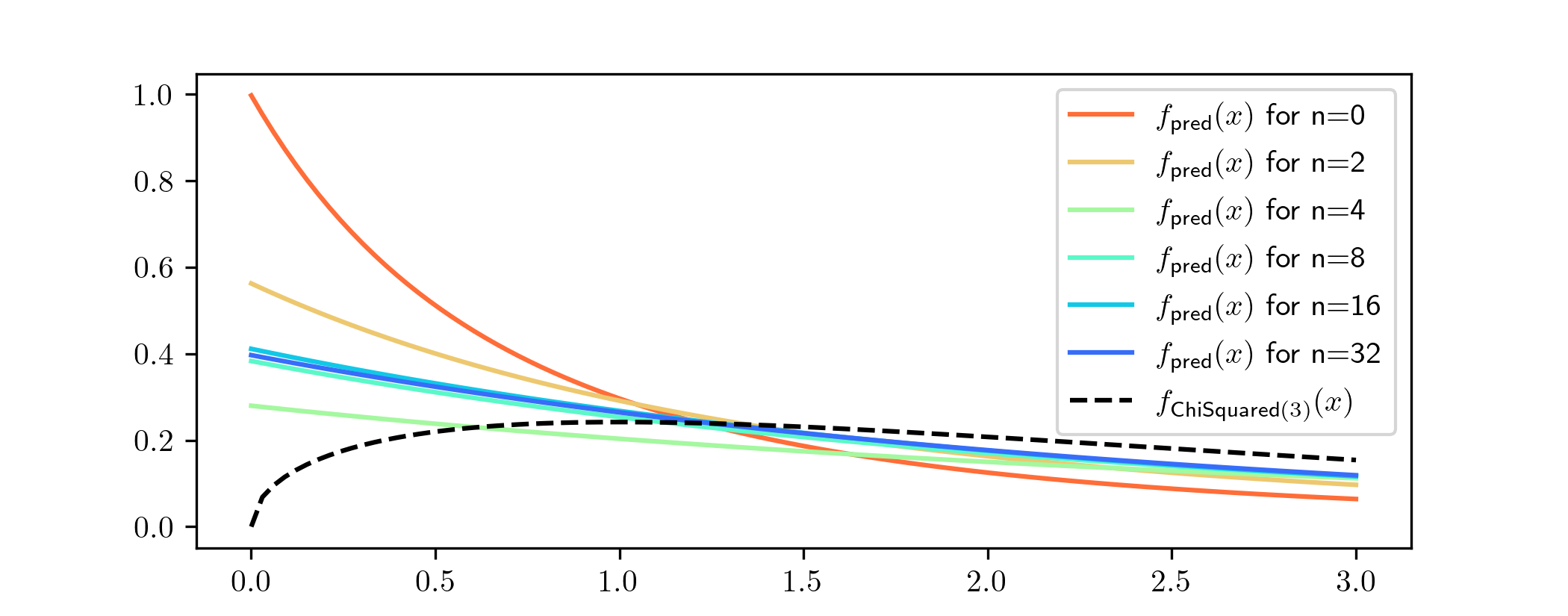
As before, it looks like our model is trying to focus in on one particular value for $\lambda $. This time it looks to be homing in on a value a little below $0.5$, although it not yet clear which. Note that the convergence appearing here actually seems faster than in Example 4.4.1 i.e. the values shown here for $n$ are a bit smaller. Let us draw the probability density functions of the predictive distributions that come from the posteriors above, and compare them to the true density function from which our data was sampled:

The density functions of the predictive distributions also seem to be converging as $n$ gets larger, as we would expect from the convergence suggested in the previous graph. But what they are converging towards is not much like the p.d.f. from which the data was actually generated (shown as the black dotted line). It puts far too much weight on small values, for example. If we hadn’t looked at these graphs we might not have noticed that anything was wrong.

In other situations, where we choose a model that is not able to represent the data well, the posterior distributions won’t converge at all as $n\to \infty $. In such cases the predictive distributions tend to be wildly wrong by comparison to the data.

What if the prior excludes the true value?

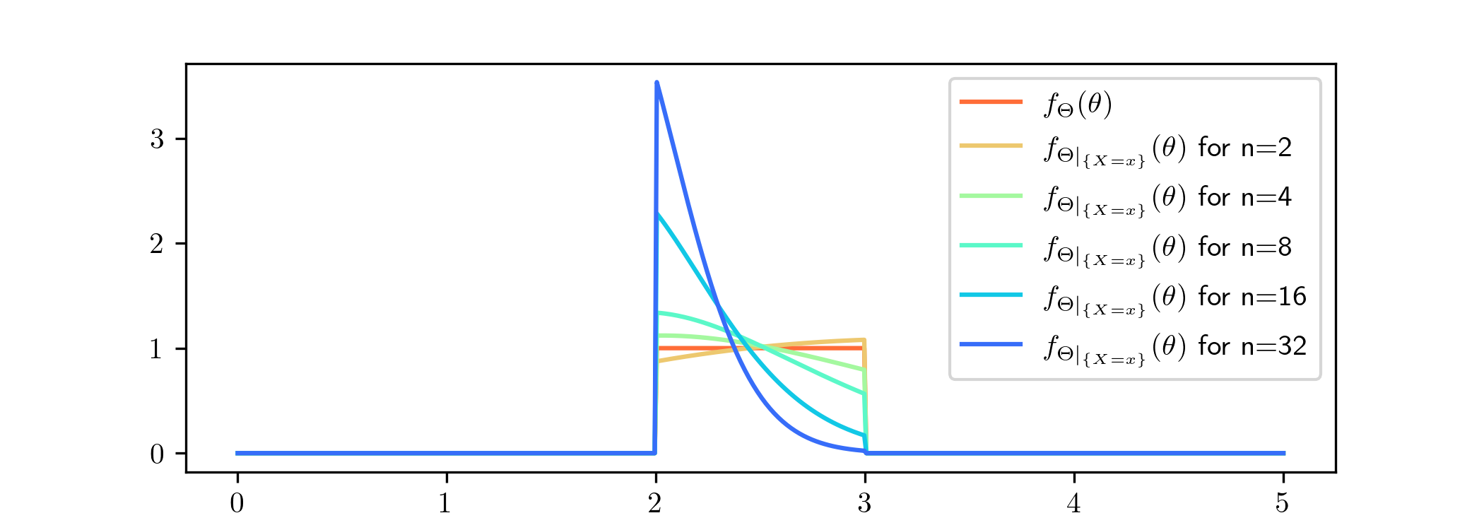
Example 4.4.3 We’ll use the model Example 4.4.1 again, but we’ll change the prior, to be $\Theta \sim \Unif ([2,3])$, the continuous uniform distribution with range $[2,3]$. We’ll feed the model data consisting of i.i.d. samples from the $\Exp (1)$ distribution, corresponding (as in Example 4.4.1) to a true value $\lambda ^*=1$ for the parameter. The key point is that in this case the true value is outside of the range of the prior. Let’s examine what happens now:

The posteriors are focusing on the value $\lambda =2$, but the most conspicuous feature is that the posterior distributions place no weight at all outside of $[2,3]$. In fact we knew this in advance, because Theorems 2.4.1 and 3.1.2 both include the fact that the range of $\Theta |_{\{X=x\}}$ is equal to the range of $\Theta $, in this case $[2,3]$. This means that, no matter how much data we give to our model, it will never converge towards the true value $\lambda ^*=1$. It is trying to do the next best thing, and get as close as possible. We won’t draw the predictive distributions for this case, but the same story applies there.

There is an important message to take away from this example. When we assign zero prior probability to some region of the parameter space, our model interprets it as an instruction that we do not ever want to consider parameters in that region, even if it later turns out that the data fits that region better. If we chose to do this based on our own (or our expert colleagues) opinions, and it turns out that we are wrong, then we have made a serious error.

To avoid that situation, it is generally agreed that the range of the prior should include all values of the parameter that are physically possible, with a view to the situation that we are trying to model. This is known as Cromwell’s rule, based on the quotation

I beseech you, in the bowels of Christ, think it possible that you may be mistaken!

which Oliver Cromwell famously wrote in a letter to the council of the Church of Scotland in 1650, in an attempt to persuade them not to support an invasion of England. Cromwell failed to persuade them and shortly afterwards Scotland did invade England. Cromwell’s own forces decisively won the resulting battle for the English side.

We have followed Cromwell’s rule in Example 2.3.3, where the parameter $p$ represented a probability and our prior had range $[0,1]$. Similarly, in Example 4.2.4 the parameter $\theta $ represented a speed and our prior had range $\R $. In the context of that example we would hope that negative values of the parameter would not be plausible (or the speed camera is seriously malfunctioning!) but we still allowed, in our prior, a small probability that this might occur.