Bayesian Statistics
4.5 The normal distribution with unknown mean and variance
We’ve considered the normal distribution with a fixed variance, but with unknown mean, in Lemma 4.2.2 and Example 4.2.4. The situation of fixed mean and unknown variance is treated in Exercise 4.4. We’ll deal here with the case where both the mean and variance are unknown parameters.
In the formulae obtained in Lemma 4.2.2, both variables relating the variance (\(\sigma ^2\) and \(s^2\)) only appeared as \(\frac {1}{\sigma ^2}\) and \(\frac {1}{s^2}\). This suggests that we would obtain neater formulae if we parameterized the variance part as \(\tau =\frac {1}{\sigma ^2}\). The parameter \(\tau \) is known as precision. We will use this form in the next lemma, and also in Exercise 4.4.
The conjugate prior in this case is complicated. It is the Normal-Gamma distribution, written \(\NGam (m,p,a,b)\) with p.d.f.
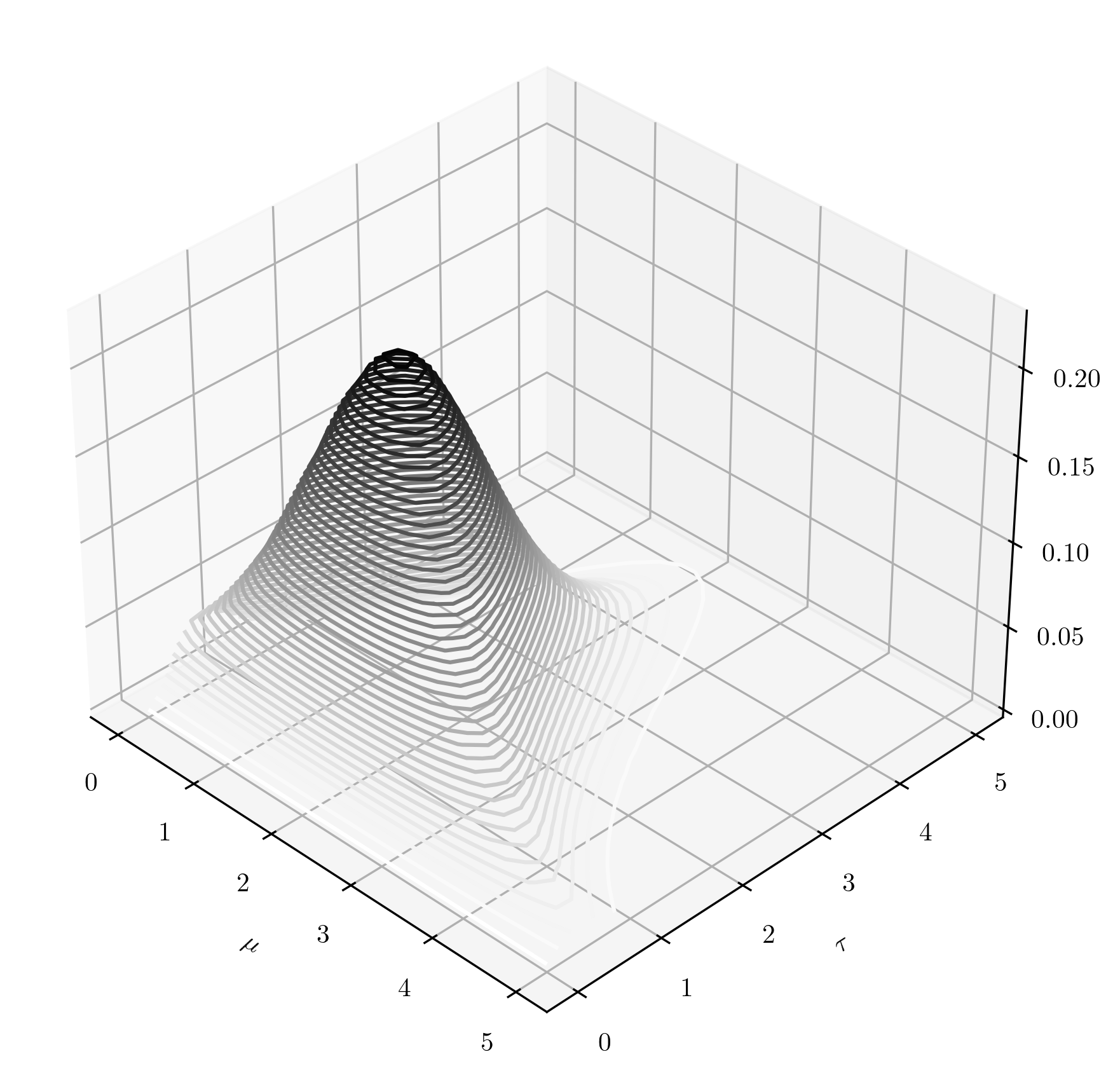
\(\seteqnumber{0}{4.}{7}\)\begin{align} f_{\NGam (m,p,a,b)}(\mu ,\tau ) \;&=\;f_{\Normal (m,\frac {1}{p\tau })}(\mu )\, f_{\Gam (a,b)}(\tau ) \label {eq:NGamma_pre} \\ &=\; \sqrt {\frac {p\tau }{2\pi }}\exp \l (-\frac {p\tau }{2}(\mu -m)^2\r )\;\; \frac {b^a}{\Gamma (a)}\tau ^{a-1}e^{-b\tau } \notag \\ &\;\propto \tau ^{a-\frac 12}\exp \l (-\frac {p\tau }{2}(\mu -m)^2-b\tau \r ). \label {eq:NGamma} \end{align} You can find this p.d.f. on the reference sheets in Appendix A. Note that it is a two-dimensional distribution, which we will use to construct random versions of the parameters \(\mu \) and \(\tau \) in \(\Normal (\mu ,\frac {1}{\tau })\). The restrictions on the \(\NGam \) parameters are that \(m\in \R \) and \(p,a,b>0\). The range is \(\mu \in \R \) and \(\tau >0\). Here’s a contour plot of the p.d.f. of \(\NGam (2,1,3,2)\) to give some idea of what is going on here:
Let us note a couple of facts about the \(\NGam (m,p,a,b)\) distribution before we proceed further. If \((U,T)\sim \NGam (m,p,a,b)\) then:
-
• The marginal distribution of \(T\) is \(\Gam (a,b)\).
This follows easily from (4.8). Integrating out \(\mu \) will remove the term \(f_{\Normal (m,\frac {1}{p\tau })}(\mu )\), which is a p.d.f. and integrates to \(1\), leaving only term \(f_{\Gam (a,b)}(\tau )\).
-
• The conditional distribution of \(U|_{\{T=\tau \}}\) is \(\Normal (m,\frac {1}{p\tau })\).
This also follows from (4.8), by applying Lemma 1.6.1. We already know that \(f_T(t)=f_{\Gam (a,b)}(\tau )\), so
\[f_{U|_{\{T=\tau \}}}(\mu )=\frac {f_{\Normal (m,\frac {1}{p\tau })}(\mu )\, f_{T}(\tau )}{f_{T}(\tau )}=f_{\Normal (m,\frac {1}{p\tau })}(\mu ).\]
Note that we are using \(U\) as a capital \(\mu \) and \(T\) as a capital \(\tau \), to preserve our usual relationship between random variables and the arguments of their probability density functions. These two facts won’t be used in our proof of conjugacy, but hopefully they help explain the formula (4.8) and the picture below it.
Our next goal is to state the conjugacy between \(\NGam \) and the Normal distribution. We will need the sample-mean-variance identity, which states that for all \(x\in \R ^n\)
\(\seteqnumber{0}{4.}{9}\)\begin{equation} \label {eq:sample-mean-variance} \sum _{i=1}^n(x_i-\mu )^2=ns^2 + n(\bar {x}-\mu )^2 \end{equation}
where \(\bar {x}=\frac {1}{n}\sum _{1}^n x_i\) and \(s^2=\frac {1}{n}\sum _{1}^n(x_i-\bar {x})^2\).
-
Remark 4.5.1 \(\offsyl \) To deduce (4.10), let \(Z\) be a random variable with the uniform distribution on \(\{x_1,\ldots ,x_n\}\). Note that \(\E [Z]=\bar {x}\) and \(\var (Z)=s^2\). The identity follows from the fact that \(\var (Z)=\var (Z-\mu )=\E [(Z-\mu )^2]-\E [Z-\mu ]^2\).
-
Lemma 4.5.2 (Normal-NGamma conjugate pair) Let \((X,\Theta )\) be a continuous Bayesian model with model family \(M_{\mu ,\tau }\sim \Normal (\mu ,\frac {1}{\tau })^{\otimes n}\), with parameters \(\mu \in \R \) and \(\tau >0\). Suppose that the prior is \(\Theta =(U,T)\sim \NGam (m,p,a,b)\) and let \(x\in \R ^n\). Then \(\Theta |_{\{X=x\}}\sim \NGam \l (m^*,p^*,a^*,b^*\r )\) where
\[\begin {alignedat}{2} m^* &= \frac {n\bar {x}+mp}{n+p} \qquad \qquad && p^* = n+p \\ a^* &= a + \frac {n}{2} && b^* = b + \frac {n}{2}\l (s^2+\frac {p}{n+p}\l (\bar {x}-m\r )^2\r ), \end {alignedat}\]
where \(\bar {x}=\frac {1}{n}\sum _1^n x_i\) and \(s^2=\frac 1n\sum _1^n (x_i-\bar {x})^2\).
Proof: \(\offsyl \) From Theorem 3.1.2 we have that for all \(\mu \in \R \) and \(\tau >0\),
\(\seteqnumber{0}{4.}{10}\)\begin{align*} f_{(U,T)|_{\{X=x\}}}(\mu ,\tau ) &\propto \l (\prod _{i=1}^n\sqrt {\frac {\tau }{2\pi }}\exp \l (-\frac {\tau (\mu -x_i)^2}{2}\r )\r ) \tau ^{a-\frac 12}\exp \l (-\frac {p\tau }{2}(\mu -m)^2-b\tau \r ) \\ &\propto \tau ^{\frac {n}{2}+a-\frac 12}\exp \l [-\frac {\tau }{2}\l (\sum _{i=1}^n(\mu -x_i)^2 + p(\mu -m)^2+2b\r )\r ] \\ &\propto \tau ^{\frac {n}{2}+a-\frac 12}\exp \l [-\frac {\tau }{2}\l (ns^2+n(\mu -\bar {x})^2 + p(\mu -m)^2+2b\r )\r ] \\ &\propto \tau ^{\frac {n}{2}+a-\frac 12}\exp \l [-\frac {\tau }{2}\mc {Q}(\mu )\r ] \end{align*} To deduce the third line we have used (4.10). We have
\[\mc {Q}(\mu )= \mu ^2 \stackrel {A}{\overbrace {\l (n+p\r )}} -2\mu \stackrel {B}{\overbrace {\l (n\bar {x} +mp\r )}} + \stackrel {C}{\overbrace {\l (ns^2 + n\bar {x}^2+pm^2+2b\r )}}.\]
Completing the square (with the help of the reference sheet) we obtain \(\mc {Q}(\mu )=A(\mu -\frac {B}{A})^2+C-\frac {B^2}{A}\) and hence
\(\seteqnumber{0}{4.}{10}\)\begin{align*} f_{(U,T)|_{\{X=x\}}}(\mu ,\tau ) &\propto \tau ^{\frac {n}{2}+a-\frac 12}\exp \l [-\frac {\tau }{2}A\l (\mu -\frac {B}{A}\r )^2-\tau \frac {1}{2}\l (C-\frac {B^2}{A}\r )\r ]. \end{align*} The right hand side is above in the form of (4.9) and we can now extract the posterior \(\NGam \) parameters. From the exponent of \(\tau \) we have \(a^*=a+\frac {n}{2}\). From the term \((\mu -\ldots )^2\) we have \(m^*=\frac {B}{A}=\frac {n\bar {x}+mp}{n+p}\) and from the coefficient of this term we have \(p^*=A=n+p\). This leaves only
\(\seteqnumber{0}{4.}{10}\)\begin{align*} b^* &=\frac {1}{2}\l (C-\frac {B^2}{A}\r ) \\ &=\frac {1}{2}\l [ns^2 + n\bar {x}^2+pm^2+2b-\frac {1}{n+p}\l (n\bar {x}+mp\r )^2\r ] \\ &=b+\frac {ns^2}{2}+\frac {1}{n+p}\l [(n+p)n\bar {x}^2+(n+p)pm^2-n^2\bar {x}^2+2mpn\bar {x}-m^2p^2\r ] \\ &=b+\frac {ns^2}{2}+\frac {1}{n+p}\l [pn\bar {x}^2+npm^2+2mpn\bar {x}\r ] \\ &=b+\frac {ns^2}{2}+\frac {np}{n+p}(\bar {x}-m)^2, \end{align*} which completes the proof. ∎
-
Example 4.5.3 Coming back to Example 4.2.4, regarding testing a speed camera, we can now do a Bayesian update where both the mean and variance are unknown parameters.
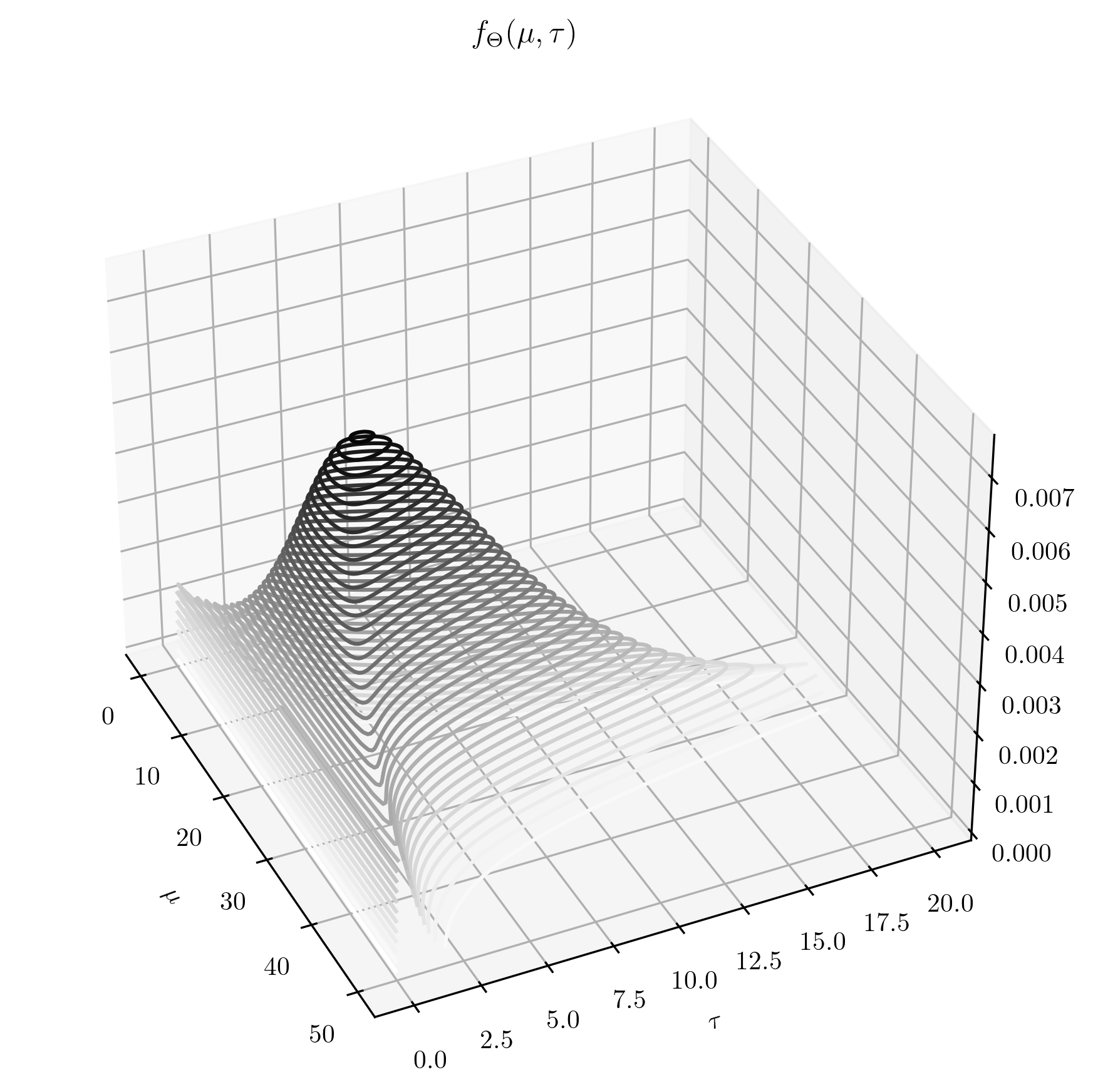
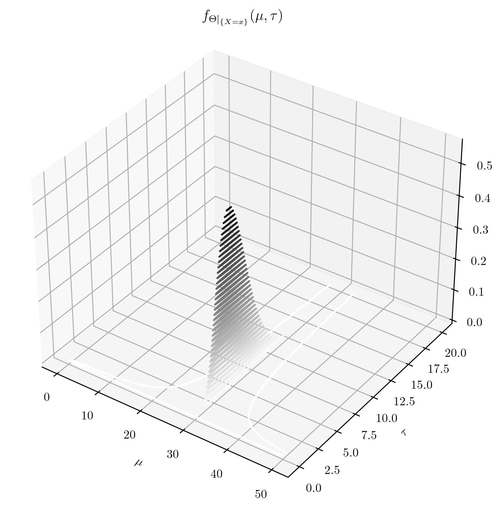
On the left we’ve taken an \(\NGam (30,\frac {1}{10^2},1,\frac 15)\) prior. Note that \(p=\frac {1}{10^2}\) corresponds to standard deviation \(=10\), so our prior is well spread out about its mean \(m=\mu =30\) on the \(\mu \)-axis. The values chosen for \(a\) and \(b\) ensure that the prior is also well spread out on the \(\tau \)-axis. On the right we have the resulting \(\NGam (30.14, 10.01, 6.00, 1.24)\) posterior. These posterior parameters were computing using Lemma 4.5.2 and with the same ten datapoints as in Example 4.2.4. As we would expect from Example 4.2.4, the mass of the posterior has focused close to \(\mu \approx 30\). The parameter \(\tau \) has focused on a wide range of fairly large values, but remember that \(\tau =\frac {1}{\sigma ^2}\) so the range of likely values for the standard deviation \(\sigma \) will in fact be a small range of small numbers.
Comparing the predictive densities gives:
Our new predictive distribution is still broadly similar to the manufacturers \(\Normal (30,0.16)\) claim, but it now looks more spread out and the mean remains slightly higher than the manufacturers claim. A point that might worry us is that our new predictive p.d.f. is not close to zero at 31mph, whereas the manufacturer claims that it should be; our data suggests that the camera is more likely to overestimate speeds than the manufacturer has claimed. We can’t reasonably say more without statistical testing, which we’ll study in Chapter 7.
Think for a moment about how much numerical work has been done to produce a graph of the predictive pdf here. According to (3.5), for each point \(x'\) on the graph, to obtain \(f_{\text {pred}}(x')\) we need to integrate \(f_{\Normal (\mu ,\frac {1}{\tau })}(x')f_{\NGam (30.14, 10.01, 6.00, 1.24)}(\mu ,\tau )\) with respect to both \(\mu \) and \(\tau \), over a region of \(\R ^2\) that includes the spike visible on the posterior density. Numerical integration over \(\R ^2\) is expensive – doing it once is not very noticeable, but doing it repeatedly usually is. The graph was made using \(30\) \(x\)-axis values and took \(255\) seconds to create, using scipy.integrate.dblquad for the integration. If we had three unknown parameters then we would have to integrate in \(\R ^3\), which is even worse. In fact, problems of this type with several parameters quickly become computationally infeasible via direct numerical integration. They need a more subtle numerical technique, which we’ll introduce in Chapter 8.


